- Python Pandas - Basics
- Python Pandas - Introduction to Data Structures
- Python Pandas - Index Objects
- Python Pandas - Panel
- Python Pandas - Basic Functionality
- Python Pandas - Indexing & Selecting Data
- Python Pandas - Series
- Python Pandas - Series
- Python Pandas - Slicing a Series Object
- Python Pandas - Attributes of a Series Object
- Python Pandas - Arithmetic Operations on Series Object
- Python Pandas - Converting Series to Other Objects
- Python Pandas - DataFrame
- Python Pandas - DataFrame
- Python Pandas - Accessing DataFrame
- Python Pandas - Slicing a DataFrame Object
- Python Pandas - Modifying DataFrame
- Python Pandas - Removing Rows from a DataFrame
- Python Pandas - Arithmetic Operations on DataFrame
- Python Pandas - IO Tools
- Python Pandas - IO Tools
- Python Pandas - Working with CSV Format
- Python Pandas - Reading & Writing JSON Files
- Python Pandas - Reading Data from an Excel File
- Python Pandas - Writing Data to Excel Files
- Python Pandas - Working with HTML Data
- Python Pandas - Clipboard
- Python Pandas - Working with HDF5 Format
- Python Pandas - Comparison with SQL
- Python Pandas - Data Handling
- Python Pandas - Sorting
- Python Pandas - Reindexing
- Python Pandas - Iteration
- Python Pandas - Concatenation
- Python Pandas - Statistical Functions
- Python Pandas - Descriptive Statistics
- Python Pandas - Working with Text Data
- Python Pandas - Function Application
- Python Pandas - Options & Customization
- Python Pandas - Window Functions
- Python Pandas - Aggregations
- Python Pandas - Merging/Joining
- Python Pandas - MultiIndex
- Python Pandas - Basics of MultiIndex
- Python Pandas - Indexing with MultiIndex
- Python Pandas - Advanced Reindexing with MultiIndex
- Python Pandas - Renaming MultiIndex Labels
- Python Pandas - Sorting a MultiIndex
- Python Pandas - Binary Operations
- Python Pandas - Binary Comparison Operations
- Python Pandas - Boolean Indexing
- Python Pandas - Boolean Masking
- Python Pandas - Data Reshaping & Pivoting
- Python Pandas - Pivoting
- Python Pandas - Stacking & Unstacking
- Python Pandas - Melting
- Python Pandas - Computing Dummy Variables
- Python Pandas - Categorical Data
- Python Pandas - Categorical Data
- Python Pandas - Ordering & Sorting Categorical Data
- Python Pandas - Comparing Categorical Data
- Python Pandas - Handling Missing Data
- Python Pandas - Missing Data
- Python Pandas - Filling Missing Data
- Python Pandas - Interpolation of Missing Values
- Python Pandas - Dropping Missing Data
- Python Pandas - Calculations with Missing Data
- Python Pandas - Handling Duplicates
- Python Pandas - Duplicated Data
- Python Pandas - Counting & Retrieving Unique Elements
- Python Pandas - Duplicated Labels
- Python Pandas - Grouping & Aggregation
- Python Pandas - GroupBy
- Python Pandas - Time-series Data
- Python Pandas - Date Functionality
- Python Pandas - Timedelta
- Python Pandas - Sparse Data Structures
- Python Pandas - Sparse Data
- Python Pandas - Visualization
- Python Pandas - Visualization
- Python Pandas - Additional Concepts
- Python Pandas - Caveats & Gotchas
- Python Pandas Useful Resources
- Python Pandas - Quick Guide
- Python Pandas - Cheatsheet
- Python Pandas - Useful Resources
- Python Pandas - Discussion
Python Pandas - Quick Guide
Python Pandas - Introduction
Pandas is an open-source Python Library providing high-performance data manipulation and analysis tool using its powerful data structures. The name Pandas is derived from the word Panel Data an Econometrics from Multidimensional data.
In 2008, developer Wes McKinney started developing pandas when in need of high performance, flexible tool for analysis of data.
Prior to Pandas, Python was majorly used for data munging and preparation. It had very little contribution towards data analysis. Pandas solved this problem. Using Pandas, we can accomplish five typical steps in the processing and analysis of data, regardless of the origin of data load, prepare, manipulate, model, and analyze.
Python with Pandas is used in a wide range of fields including academic and commercial domains including finance, economics, Statistics, analytics, etc.
Key Features of Pandas
- Fast and efficient DataFrame object with default and customized indexing.
- Tools for loading data into in-memory data objects from different file formats.
- Data alignment and integrated handling of missing data.
- Reshaping and pivoting of date sets.
- Label-based slicing, indexing and subsetting of large data sets.
- Columns from a data structure can be deleted or inserted.
- Group by data for aggregation and transformations.
- High performance merging and joining of data.
- Time Series functionality.
Python Pandas - Environment Setup
Setting up an environment to use the Pandas library is straightforward, and there are multiple ways to achieve this. Whether you prefer using Anaconda, Miniconda, or pip, you can easily get Pandas up and running on your system. This tutorial will guide you through the different methods to install Pandas.
Installing Pandas with pip
The most common way to install Pandas is by using the pip, it is a Python package manager (pip) allows you to install modules and packages. This method is suitable if you already have Python installed on your system. Note that the standard Python distribution does not come bundled with the Pandas module.
To install the pandas package by using pip you need to open the command prompt in our system (assuming, your machine is a windows operating system), and run the following command −
pip3 install pandas
This command will download and install the Pandas package along with its dependencies. If you install Anaconda Python package, Pandas will be installed by default with the following −
Upgrading pip (if necessary)
If you encounter any errors regarding the pip version, you can upgrade pip using the following command −
python -m pip3 install --upgrade pip
Then, rerun the Pandas installation command.
Installing a Specific Version of Pandas
If you need a specific version of Pandas, you can specify it using the following command −
pip3 install pandas==2.3.3
Every time, when you try to install any package, initially pip will check for the package dependencies if they are already installed on the system or not. if not, it will install them. Once all dependencies have been satisfied, it proceeds to install the requested package(s).
Installing Pandas Using Anaconda
Anaconda is a popular distribution for data science that includes Python and many scientific libraries, including Pandas.
Following are the steps to install Anaconda −
- Download Anaconda: Go to Anaconda's official website and download the installer suitable for your operating system.
- Install Anaconda: Follow the installation instructions provided on the Anaconda website.
Pandas comes pre-installed with Anaconda, so you can directly import it in your Python environment.
import pandas as pd
Installing a Specific Version of Pandas with Anaconda
If you need a specific version of Pandas, you can install it using the conda command −
conda install pandas=2.3.3
Anaconda will take up to 300GB of system space for storage and 600GB for air-gapped deployments because it comes with the most common data science packages in Python like Numpy, Pandas, and many more.
Installing Pandas Using Miniconda
Both Anaconda and minconda use the conda package installer, but using anaconda will occupy more system storage. Because anaconda has more than 100 packages, those are automatically installed and the result needs more space.
Miniconda is a minimal installer for conda, which includes only the conda package manager and Python. It is lightweight compared to Anaconda and is suitable if you want more control over the packages you install.
Following are the steps to install Miniconda −
- Download Miniconda: Visit the Miniconda download page and download the installer for your operating system.
- Install Miniconda: Follow the installation instructions provided on the Miniconda website.
Installing Pandas with Miniconda
After successfully installing Miniconda, you can use the conda command to install Pandas −
conda install pandas
Installing Pandas on Linux
On Linux, you can use the package manager of your respective distribution to install Pandas and other scientific libraries.
For Ubuntu Users
sudo apt-get install python-numpy python-scipy python-matplotlibipythonipythonnotebook
python-pandas python-sympy python-nose
For Fedora Users
sudo yum install numpyscipy python-matplotlibipython python-pandas sympy
python-nose atlas-devel
By following any of these methods, you can set up Pandas on your system and start using it for data analysis and manipulation.
Python Pandas - Introduction to Data Strutures
Python Pandas Data Structures
Data structures in Pandas are designed to handle data efficiently. They allow for the organization, storage, and modification of data in a way that optimizes memory usage and computational performance. Python Pandas library provides two primary data structures for handling and analyzing data −
- Series
- DataFrame
In general programming, the term "data structure" refers to the method of collecting, organizing, and storing data to enable efficient access and modification. Data structures are collections of data types that provide the best way of organizing items (values) in terms of memory usage.
Pandas is built on top of NumPy and integrates well within a scientific computing environment with many other third-party libraries. This tutorial will provide a detailed introduction to these data structures.
Dimension and Description of Pandas Data Structures
| Data Structure | Dimensions | Description |
|---|---|---|
| Series | 1 | A one-dimensional labeled homogeneous array, sizeimmutable. |
| Data Frames | 2 | A two-dimensional labeled, size-mutable tabular structure with potentially heterogeneously typed columns. |
Working with two or more dimensional arrays can be complex and time-consuming, as users need to carefully consider the data's orientation when writing functions. However, Pandas simplifies this process by reducing the mental effort required. For example, when dealing with tabular data (DataFrame), it's more easy to think in terms of rows and columns instead of axis 0 and axis 1.
Mutability of Pandas Data Structures
All Pandas data structures are value mutable, meaning their contents can be changed. However, their size mutability varies −
- Series − Size immutable.
- DataFrame − Size mutable.
Series
A Series is a one-dimensional labeled array that can hold any data type. It can store integers, strings, floating-point numbers, etc. Each value in a Series is associated with a label (index), which can be an integer or a string.
| Name | Steve |
| Age | 35 |
| Gender | Male |
| Rating | 3.5 |
Example
Consider the following Series which is a collection of different data types
import pandas as pd

data = ['Steve', '35', 'Male', '3.5']
series = pd.Series(data, index=['Name', 'Age', 'Gender', 'Rating'])
print(series)
On executing the above program, you will get the following output −
Name      Steve
Age          35
Gender     Male
Rating      3.5
dtype: object
Key Points
Following are the key points related to the Pandas Series.
- Homogeneous data
- Size Immutable
- Values of Data Mutable
DataFrame
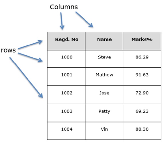
A DataFrame is a two-dimensional labeled data structure with columns that can hold different data types. It is similar to a table in a database or a spreadsheet. Consider the following data representing the performance rating of a sales team −
| Name | Age | Gender | Rating |
|---|---|---|---|
| Steve | 32 | Male | 3.45 |
| Lia | 28 | Female | 4.6 |
| Vin | 45 | Male | 3.9 |
| Katie | 38 | Female | 2.78 |
Example
The above tabular data can be represented in a DataFrame as follows −
import pandas as pd

# Data represented as a dictionary
data = {
    'Name': ['Steve', 'Lia', 'Vin', 'Katie'],
    'Age': [32, 28, 45, 38],
    'Gender': ['Male', 'Female', 'Male', 'Female'],
    'Rating': [3.45, 4.6, 3.9, 2.78]
}

# Creating the DataFrame
df = pd.DataFrame(data)

# Display the DataFrame
print(df)
Output
On executing the above code you will get the following output −
    Name  Age  Gender  Rating
0  Steve   32    Male    3.45
1    Lia   28  Female    4.60
2    Vin   45    Male    3.90
3  Katie   38  Female    2.78
Key Points
Following are the key points related the Pandas DataFrame −
- Heterogeneous data
- Size Mutable
- Data Mutable
Purpose of Using More Than One Data Structure
Pandas data structures are flexible containers for lower-dimensional data. For instance, a DataFrame is a container for Series, and a Series is a container for scalars. This flexibility allows for efficient data manipulation and storage.
Building and handling multi-dimensional arrays can be boring and require careful consideration of the data's orientation when writing functions. Pandas reduces this mental effort by providing intuitive data structures.
Example
Following example represents a Series within a DataFrame.
import pandas as pd

# Data represented as a dictionary
data = {
    'Name': ['Steve', 'Lia', 'Vin', 'Katie'],
    'Age': [32, 28, 45, 38],
    'Gender': ['Male', 'Female', 'Male', 'Female'],
    'Rating': [3.45, 4.6, 3.9, 2.78]
}

# Creating the DataFrame
df = pd.DataFrame(data)

# Display a Series within a DataFrame
print(df['Name'])
Output
On executing the above code you will get the following output −
0    Steve
1      Lia
2      Vin
3    Katie
Name: Name, dtype: object
Python Pandas - Index Objects
In Pandas, Index Objects play an important role in organizing and accessing data in a structured way. They work like labeled arrays and play an important role in defining how data is arranged and accessed in structures like Series and DataFrames. The Index allows quick data searches, efficient slicing, and keeps data properly aligned, while giving each row meaningful labels.
An Index is used to label the rows of a DataFrame or elements in a Series. These labels can be numbers, strings, or dates, and they help you to identify the data. One key thing to remember about Pandas indexes is that they are immutable, meaning you cannot change their size once created.
In this tutorial, we will learn about Pandas Index Objects, and various types of indexes in pandas.
The Index Class
The Index class is a basic object for storing all index types in Pandas objects. It provides the basic functionality for accessing and manipulating data.
Key Features of Index Object
Immutable: Index object is a immutable sequence, which cannot modify once it is created.
Alignment: Index ensures that data from different DataFrames or Series can be combined correctly, based on the index values.
Slicing: Index allows fast slicing and retrieval of data based on labels.
Syntax
Following is the syntax of the Index class −
class pandas.Index(data=None, dtype=None, copy=False, name=None, tupleize_cols=True)
Where,
data: The data for the index, which can be an array-like structure (like a list or numpy array) or another index object.
dtype: It specifies the data type for the index values, If not provided, Pandas will decide the data type based on the index values.
copy: It is a boolean parameter (True or False), which, specifies to create a copy of the input data.
name: This parameter gives a label to the index.
data: It is also a boolean parameter (True or False), When True, it tries to create MultiIndex if possible.
Types of Indexes in Pandas
Pandas provides various types of indexes to handle different types of data. Such as −
Let's discuss about all types of indexes in pandas.
NumericIndex
A NumericIndex is the basic index type in Pandas, it contains numerical values. NumericIndex is a default index and Pandas automatically assigns this if you did not provided any index.
Example
Following example demonstrates how pandas automatically assigns NumericIndex to a pandas DataFrame object.
import pandas as pd

# Generate some data for DataFrame
data = {
   'Name': ['Steve', 'Lia', 'Vin', 'Katie'],
   'Age': [32, 28, 45, 38],
   'Gender': ['Male', 'Female', 'Male', 'Female'],
   'Rating': [3.45, 4.6, 3.9, 2.78]
}
# Creating the DataFrame
df = pd.DataFrame(data)

# Display the DataFrame
print(df)

print("\nDataFrame Index Object Type:",df.index.dtype)
Output
Following is the output of the above code −
    Name  Age  Gender  Rating
0  Steve   32    Male    3.45
1    Lia   28  Female    4.60
2    Vin   45    Male    3.90
3  Katie   38  Female    2.78

DataFrame Index Object Type: int64
Categorical Index
The CategoricalIndex is used to deal the duplicate labels. This index is efficient in terms of memory usage and handling the large number of duplicate elements.
Example
The Following example create a Pandas DataFrame with the CategoricalIndex.
import pandas as pd

# Creating a CategoricalIndex
categories = pd.CategoricalIndex(['a','b', 'a', 'c'])
df = pd.DataFrame({'Col1': [50, 70, 90, 60], 'Col2':[1, 3, 5, 8]}, index=categories)
print("Input DataFrame:\n",df)

print("\nDataFrame Index Object Type:",df.index.dtype)
Output
Following is the output of the above code −
Input DataFrame:
    Col1  Col2
a    50     1
b    70     3
a    90     5
c    60     8

DataFrame Index Object Type: category
IntervalIndex
An IntervalIndex is used to represent intervals (ranges) in your data. This type of index will be created using the interval_range() method.
Example
Following example creates a DataFrame with IntervalIndex using the interval_range() method.
import pandas as pd

# Creating a IntervalIndex
interval_idx = pd.interval_range(start=0, end=4)

# Creating a DataFrame with IntervalIndex
df = pd.DataFrame({'Col1': [1, 2, 3, 4], 'Col2':[1, 3, 5, 8]}, index=interval_idx)

print("Input DataFrame:\n",df)

print("\nDataFrame Index Object Type:",df.index.dtype)
Output
Following is the output of the above code −
Input DataFrame:
         Col1  Col2
(0, 1]     1     1
(1, 2]     2     3
(2, 3]     3     5
(3, 4]     4     8

DataFrame Index Object Type: interval[int64, right]
MultiIndex
Pandas MultiIndex is used to represent multiple levels or layers in index of Pandas data structures, which is also called as hierarchical.
Example
The following example shows the creation of a simple MultiIndexed DataFrame.
import pandas as pd

# Create MultiIndex
arrays = [[1, 1, 2, 2], ['red', 'blue', 'red', 'blue']]
multi_idx = pd.MultiIndex.from_arrays(arrays, names=('number', 'color'))

# Create a DataFrame with MultiIndex
df = pd.DataFrame({'Col1': [1, 2, 3, 4], 'Col2':[1, 3, 5, 8]}, index=multi_idx)

print("MultiIndexed DataFrame:\n",df)
Output
Following is the output of the above code −
MultiIndexed DataFrame:
               Col1  Col2
number color
1      red       1     1
       blue      2     3
2      red       3     5
       blue      4     8
DatetimeIndex
Pandas DatetimeIndex object is used to represent the date and time values. Nothing but it used for time-series data where each row is linked to a specific timestamp.
Example
The Following example create a Pandas DataFrame with the DatetimeIndex.
import pandas as pd

# Create DatetimeIndex
datetime_idx = pd.DatetimeIndex(["2020-01-01 10:00:00", "2020-02-01 11:00:00"])

# Create a DataFrame with DatetimeIndex
df = pd.DataFrame({'Col1': [1, 2], 'Col2':[1, 3]}, index=datetime_idx )

print("DatetimeIndexed DataFrame:\n",df)
Output
Following is the output of the above code −
DatetimeIndexed DataFrame:
                      Col1  Col2
2020-01-01 10:00:00     1     1
2020-02-01 11:00:00     2     3
TimedeltaIndex
Pandas TimedeltaIndex is used represent a duration between two dates or times, like the number of days or hours between events.
Example
This example creates a Pandas DataFrame with a TimedeltaIndex.
import pandas as pd

# Create TimedeltaIndex
timedelta_idx = pd.TimedeltaIndex(['0 days', '1 days', '2 days'])

# Create a DataFrame with TimedeltaIndex
df = pd.DataFrame({'Col1': [1, 2, 3], 'Col2':[1, 3, 3]}, index=timedelta_idx )

print("TimedeltaIndexed DataFrame:\n",df)
Output
Following is the output of the above code −
TimedeltaIndexed DataFrame:
         Col1  Col2
0 days     1     1
1 days     2     3
2 days     3     3
PeriodIndex
Pandas PeriodIndex is used to represent regular periods in time, like quarters, months, or years.
Example
This example creates a Pandas DataFrame with PeriodIndex object.
import pandas as pd

# Create PeriodIndex
period_idx = pd.PeriodIndex(year=[2020, 2024], quarter=[1, 3])

# Create a DataFrame with PeriodIndex
df = pd.DataFrame({'Col1': [1, 2], 'Col2':[1, 3]}, index=period_idx )

print("PeriodIndexed DataFrame:\n",df)
Output
Following is the output of the above code −
PeriodIndexed DataFrame:
         Col1  Col2
2020Q1     1     1
2024Q3     2     3
Python Pandas - Panel
A panel is a 3D container of data. The term Panel data is derived from econometrics and is partially responsible for the name pandas − pan(el)-da(ta)-s.
The Panel class is deprecated and has been removed in recent versions of pandas. The recommended way to represent 3-D data is with a MultiIndex on a DataFrame via the to_frame() method or with the xarray package. pandas provides a to_xarray() method to automate this conversion.
The names for the 3 axes are intended to give some semantic meaning to describing operations involving panel data. They are −
items: axis 0, each item corresponds to a DataFrame contained inside.
major_axis: axis 1, it is the index (rows) of each of the DataFrames.
minor_axis: axis 2, it is the columns of each of the DataFrames.
pandas.Panel()
A Panel can be created using the following constructor −
pandas.Panel(data, items, major_axis, minor_axis, dtype, copy)
The parameters of the constructor are as follows −
| Parameter | Description |
|---|---|
| data | Data takes various forms like ndarray, series, map, lists, dict, constants and also another DataFrame |
| items | axis=0 |
| major_axis | axis=1 |
| minor_axis | axis=2 |
| dtype | Data type of each column |
| copy | Copy data. Default, false |
Create Panel
A Panel can be created using multiple ways like −
- From ndarrays
- From dict of DataFrames
From 3D ndarray
# creating an empty panel
import pandas as pd
import numpy as np

data = np.random.rand(2,4,5)
p = pd.Panel(data)
print(p)
Its output is as follows −
<class 'pandas.core.panel.Panel'>
Dimensions: 2 (items) x 4 (major_axis) x 5 (minor_axis)
Items axis: 0 to 1
Major_axis axis: 0 to 3
Minor_axis axis: 0 to 4
Note: Observe the dimensions of the empty panel and the above panel, all the objects are different.
From dict of DataFrame Objects
#creating an empty panel
import pandas as pd
import numpy as np

data = {'Item1' : pd.DataFrame(np.random.randn(4, 3)),
   'Item2' : pd.DataFrame(np.random.randn(4, 2))}
p = pd.Panel(data)
print(p)
Its output is as follows −
Dimensions: 2 (items) x 4 (major_axis) x 3 (minor_axis)
Items axis: Item1 to Item2
Major_axis axis: 0 to 3
Minor_axis axis: 0 to 2
Create an Empty Panel
An empty panel can be created using the Panel constructor as follows −
#creating an empty panel
import pandas as pd
p = pd.Panel()
print(p)
Its output is as follows −
<class 'pandas.core.panel.Panel'>
Dimensions: 0 (items) x 0 (major_axis) x 0 (minor_axis)
Items axis: None
Major_axis axis: None
Minor_axis axis: None
Selecting the Data from Panel
Select the data from the panel using −
- Items
- Major_axis
- Minor_axis
Using Items
# creating an empty panel
import pandas as pd
import numpy as np
data = {'Item1' : pd.DataFrame(np.random.randn(4, 3)),
   'Item2' : pd.DataFrame(np.random.randn(4, 2))}
p = pd.Panel(data)
print(p['Item1'])
Its output is as follows −
            0          1          2
0    0.488224  -0.128637   0.930817
1    0.417497   0.896681   0.576657
2   -2.775266   0.571668   0.290082
3   -0.400538  -0.144234   1.110535
We have two items, and we retrieved item1. The result is a DataFrame with 4 rows and 3 columns, which are the Major_axis and Minor_axis dimensions.
Using major_axis
Data can be accessed using the method panel.major_axis(index).
# creating an empty panel
import pandas as pd
import numpy as np
data = {'Item1' : pd.DataFrame(np.random.randn(4, 3)),
   'Item2' : pd.DataFrame(np.random.randn(4, 2))}
p = pd.Panel(data)
print(p.major_xs(1))
Its output is as follows −
      Item1       Item2
0   0.417497    0.748412
1   0.896681   -0.557322
2   0.576657       NaN
Using minor_axis
Data can be accessed using the method panel.minor_axis(index).
# creating an empty panel
import pandas as pd
import numpy as np
data = {'Item1' : pd.DataFrame(np.random.randn(4, 3)),
   'Item2' : pd.DataFrame(np.random.randn(4, 2))}
p = pd.Panel(data)
print(p.minor_xs(1))
Its output is as follows −
       Item1       Item2
0   -0.128637   -1.047032
1    0.896681   -0.557322
2    0.571668    0.431953
3   -0.144234    1.302466
Note: Observe the changes in the dimensions.
Python Pandas - Basic Functionality
Pandas is a powerful data manipulation library in Python, providing essential tools to work with data in both Series and DataFrame formats. These two data structures are crucial for handling and analyzing large datasets.
Understanding the basic functionalities of Pandas, including its attributes and methods, is essential for effectively managing data, these attributes and methods provide valuable insights into your data, making it easier to understand and process. In this tutorial you will learn about the basic attributes and methods in Pandas that are crucial for working with these data structures.
Working with Attributes in Pandas
Attributes in Pandas allow you to access metadata about your Series and DataFrame objects. By using these attributes you can explore and easily understand the data.
Series and DataFrame Attributes
Following are the widely used attribute of the both Series and DataFrame objects −
| Sr.No. | Attribute & Description |
|---|---|
| 1 |
dtype Returns the data type of the elements in the Series or DataFrame. |
| 2 |
index Provides the index (row labels) of the Series or DataFrame. |
| 3 |
values Returns the data in the Series or DataFrame as a NumPy array. |
| 4 |
shape Returns a tuple representing the dimensionality of the DataFrame (rows, columns). |
| 5 |
ndim Returns the number of dimensions of the object. Series is always 1D, and DataFrame is 2D. |
| 6 |
size Gives the total number of elements in the object. |
| 7 |
empty Checks if the object is empty, and returns True if it is. |
| 8 |
columns Provides the column labels of the DataFrame object. |
Example
Let's create a Pandas Series and explore these attributes operation.
import pandas as pd
import numpy as np

# Create a Series with random numbers
s = pd.Series(np.random.randn(4))

# Exploring attributes
print("Data type of Series:", s.dtype)
print("Index of Series:", s.index)
print("Values of Series:", s.values)
print("Shape of Series:", s.shape)
print("Number of dimensions of Series:", s.ndim)
print("Size of Series:", s.size)
print("Is Series empty?:", s.empty)
Its output is as follows −
Data type of Series: float64
Index of Series: RangeIndex(start=0, stop=4, step=1)
Values of Series: [-1.02016329  1.40840089  1.36293022  1.33091391]
Shape of Series: (4,)
Number of dimensions of Series: 1
Size of Series: 4
Is Series empty?: False
Example
Let's look at below example and understand working of these attributes on a DataFrame object.
import pandas as pd
import numpy as np

# Create a DataFrame with random numbers
df = pd.DataFrame(np.random.randn(3, 4), columns=list('ABCD'))
print("DataFrame:")
print(df)

print("Results:")
print("Data types:", df.dtypes)
print("Index:", df.index)
print("Columns:", df.columns)
print("Values:")
print(df.values)
print("Shape:", df.shape)
print("Number of dimensions:", df.ndim)
print("Size:", df.size)
print("Is empty:", df.empty)
On executing the above code you will get the following output −
DataFrame:
          A         B         C         D
0  2.161209 -1.671807 -1.020421 -0.287065
1  0.308136 -0.592368 -0.183193  1.354921
2 -0.963498 -1.768054 -0.395023 -2.454112

Results:
Data types:
A    float64
B    float64
C    float64
D    float64
dtype: object
Index: RangeIndex(start=0, stop=3, step=1)
Columns: Index(['A', 'B', 'C', 'D'], dtype='object')
Values:
[[ 2.16120893 -1.67180742 -1.02042138 -0.28706468]
 [ 0.30813618 -0.59236786 -0.18319262  1.35492058]
 [-0.96349817 -1.76805364 -0.3950226  -2.45411245]]
Shape: (3, 4)
Number of dimensions: 2
Size: 12
Is empty: False
Exploring Basic Methods in Pandas
Pandas offers several basic methods in both the data structures, that makes it easy to quickly look at and understand your data. These methods help you get a summary and explore the details without much effort.
Series and DataFrame Methods
| Sr.No. | Method & Description |
|---|---|
| 1 |
head(n) Returns the first n rows of the object. The default value of n is 5. |
| 2 |
tail(n) Returns the last n rows of the object. The default value of n is 5. |
| 3 |
info() Provides a concise summary of a DataFrame, including the index dtype and column dtypes, non-null values, and memory usage. |
| 4 |
describe() Generates descriptive statistics of the DataFrame or Series, such as count, mean, std, min, and max. |
Example
Let us now create a Series and see the working of the Series basic methods.
import pandas as pd
import numpy as np

# Create a Series with random numbers
s = pd.Series(np.random.randn(10))

print("Series:")
print(s)

# Using basic methods
print("First 5 elements of the Series:\n", s.head())
print("\nLast 3 elements of the Series:\n", s.tail(3))
print("\nDescriptive statistics of the Series:\n", s.describe())
Its output is as follows −
Series:
0   -0.295898
1   -0.786081
2   -1.189834
3   -0.410830
4   -0.997866
5    0.084868
6    0.736541
7    0.133949
8    1.023674
9    0.669520
dtype: float64
First 5 elements of the Series:
 0   -0.295898
1   -0.786081
2   -1.189834
3   -0.410830
4   -0.997866
dtype: float64

Last 3 elements of the Series:
 7    0.133949
8    1.023674
9    0.669520
dtype: float64

Descriptive statistics of the Series:
 count    10.000000
mean     -0.103196
std       0.763254
min      -1.189834
25%      -0.692268
50%      -0.105515
75%       0.535627
max       1.023674
dtype: float64
Example
Now look at below example and understand working of the basic methods on a DataFrame object.
import pandas as pd
import numpy as np

#Create a Dictionary of series
data = {'Name':pd.Series(['Tom','James','Ricky','Vin','Steve','Smith','Jack']),
   'Age':pd.Series([25,26,25,23,30,29,23]),
   'Rating':pd.Series([4.23,3.24,3.98,2.56,3.20,4.6,3.8])}

#Create a DataFrame
df = pd.DataFrame(data)
print("Our data frame is:\n")
print(df)

# Using basic methods
print("\nFirst 5 rows of the DataFrame:\n", df.head())
print("\nLast 3 rows of the DataFrame:\n", df.tail(3))
print("\nInfo of the DataFrame:")
df.info()
print("\nDescriptive statistics of the DataFrame:\n", df.describe())
On executing the above code you will get the following output −
Our data frame is:

    Name  Age  Rating
0    Tom   25    4.23
1  James   26    3.24
2  Ricky   25    3.98
3    Vin   23    2.56
4  Steve   30    3.20
5  Smith   29    4.60
6   Jack   23    3.80

First 5 rows of the DataFrame:
     Name  Age  Rating
0    Tom   25    4.23
1  James   26    3.24
2  Ricky   25    3.98
3    Vin   23    2.56
4  Steve   30    3.20

Last 3 rows of the DataFrame:
     Name  Age  Rating
4  Steve   30     3.2
5  Smith   29     4.6
6   Jack   23     3.8

Info of the DataFrame:
<class 'pandas.core.frame.DataFrame'>
RangeIndex: 7 entries, 0 to 6
Data columns (total 3 columns):
 #   Column  Non-Null Count  Dtype
---  ------  --------------  -----
 0   Name    7 non-null      object
 1   Age     7 non-null      int64
 2   Rating  7 non-null      float64
dtypes: float64(1), int64(1), object(1)
memory usage: 296.0+ bytes

Descriptive statistics of the DataFrame:
              Age    Rating
count   7.000000  7.000000
mean   25.857143  3.658571
std     2.734262  0.698628
min    23.000000  2.560000
25%    24.000000  3.220000
50%    25.000000  3.800000
75%    27.500000  4.105000
max    30.000000  4.600000
Python Pandas - Indexing and Selecting Data
In pandas, indexing and selecting data are crucial for efficiently working with data in Series and DataFrame objects. These operations help you to slice, dice, and access subsets of your data easily.
These operations involve retrieving specific parts of your data structure, whether it's a Series or DataFrame. This process is crucial for data analysis as it allows you to focus on relevant data, apply transformations, and perform calculations.
Indexing in pandas is essential because it provides metadata that helps with analysis, visualization, and interactive display. It automatically aligns data for easier manipulation and simplifies the process of getting and setting data subsets.
This tutorial will explore various methods to slice, dice, and manipulate data using Pandas, helping you understand how to access and modify subsets of your data.
Types of Indexing in Pandas
Similar to Python and NumPy indexing ([ ]) and attribute (.) operators, Pandas provides straightforward methods for accessing data within its data structures. However, because the data type being accessed can be unpredictable, relying exclusively on these standard operators may lead to optimization challenges.
Pandas provides several methods for indexing and selecting data, such as −
Label-Based Indexing with .loc
Integer Position-Based Indexing with .iloc
Indexing with Brackets []
Label-Based Indexing with .loc
The .loc indexer is used for label-based indexing, which means you can access rows and columns by their labels. It also supports boolean arrays for conditional selection.
.loc() has multiple access methods like −
single scalar label: Selects a single row or column, e.g., df.loc['a'].
list of labels: Select multiple rows or columns, e.g., df.loc[['a', 'b']].
Label Slicing: Use slices with labels, e.g., df.loc['a':'f'] (both start and end are included).
Boolean Arrays: Filter data based on conditions, e.g., df.loc[boolean_array].
loc takes two single/list/range operator separated by ','. The first one indicates the row and the second one indicates columns.
Example 1
Here is a basic example that selects all rows for a specific column using the loc indexer.
#import the pandas library and aliasing as pd
import pandas as pd
import numpy as np

df = pd.DataFrame(np.random.randn(8, 4),
index = ['a','b','c','d','e','f','g','h'], columns = ['A', 'B', 'C', 'D'])

print("Original DataFrame:\n", df)

#select all rows for a specific column
print('\nResult:\n',df.loc[:,'A'])
Its output is as follows −
Original DataFrame:
           A         B         C         D
a  0.962766 -0.195444  1.729083 -0.701897
b -0.552681  0.797465 -1.635212 -0.624931
c  0.581866 -0.404623 -2.124927 -0.190193
d -0.284274  0.019995 -0.589465  0.914940
e  0.697209 -0.629572 -0.347832  0.272185
f -0.181442 -0.000983  2.889981  0.104957
g  1.195847 -1.358104  0.110449 -0.341744
h -0.121682  0.744557  0.083820  0.355442

Result:
 a    0.962766
b   -0.552681
c    0.581866
d   -0.284274
e    0.697209
f   -0.181442
g    1.195847
h   -0.121682
Name: A, dtype: float64
Note: The output generated will vary with each execution because the DataFrame is created using NumPy's random number generator.
Example 2
This example selecting all rows for multiple columns.
# import the pandas library and aliasing as pd
import pandas as pd
import numpy as np

df = pd.DataFrame(np.random.randn(8, 4),
index = ['a','b','c','d','e','f','g','h'], columns = ['A', 'B', 'C', 'D'])

# Select all rows for multiple columns, say list[]
print(df.loc[:,['A','C']])
Its output is as follows −
            A           C
a    0.391548    0.745623
b   -0.070649    1.620406
c   -0.317212    1.448365
d   -2.162406   -0.873557
e    2.202797    0.528067
f    0.613709    0.286414
g    1.050559    0.216526
h    1.122680   -1.621420
Example 3
This example selects the specific rows for the specific columns.
# import the pandas library and aliasing as pd
import pandas as pd
import numpy as np

df = pd.DataFrame(np.random.randn(8, 4),
index = ['a','b','c','d','e','f','g','h'], columns = ['A', 'B', 'C', 'D'])

# Select few rows for multiple columns, say list[]
print(df.loc[['a','b','f','h'],['A','C']])
Its output is as follows −
           A          C
a   0.391548   0.745623
b  -0.070649   1.620406
f   0.613709   0.286414
h   1.122680  -1.621420
Example 4
The following example selecting a range of rows for all columns using the loc indexer.
# import the pandas library and aliasing as pd
import pandas as pd
import numpy as np

df = pd.DataFrame(np.random.randn(8, 4),
index = ['a','b','c','d','e','f','g','h'], columns = ['A', 'B', 'C', 'D'])

# Select range of rows for all columns
print(df.loc['c':'e'])
Its output is as follows −
          A         B         C         D
c  0.044589  1.966278  0.894157  1.798397
d  0.451744  0.233724 -0.412644 -2.185069
e -0.865967 -1.090676 -0.931936  0.214358
Integer Position-Based Indexing with .iloc
The .iloc indexer is used for integer-based indexing, which allows you to select rows and columns by their numerical position. This method is similar to standard python and numpy indexing (i.e. 0-based indexing).
Single Integer: Selects data by its position, e.g., df.iloc[0].
List of Integers: Select multiple rows or columns by their positions, e.g., df.iloc[[0, 1, 2]].
Integer Slicing: Use slices with integers, e.g., df.iloc[1:3].
Boolean Arrays: Similar to .loc, but for positions.
Example 1
Here is a basic example that selects 4 rows for the all column using the iloc indexer.
# import the pandas library and aliasing as pd
import pandas as pd
import numpy as np

df = pd.DataFrame(np.random.randn(8, 4), columns = ['A', 'B', 'C', 'D'])

print("Original DataFrame:\n", df)

# select all rows for a specific column
print('\nResult:\n',df.iloc[:4])
Its output is as follows −
Original DataFrame:
           A         B         C         D
0 -1.152267  2.206954 -0.603874  1.275639
1 -0.799114 -0.214075  0.283186  0.030256
2 -1.823776  1.109537  1.512704  0.831070
3 -0.788280  0.961695 -0.127322 -0.597121
4  0.764930 -1.310503  0.108259 -0.600038
5 -1.683649 -0.602324 -1.175043 -0.343795
6  0.323984 -2.314158  0.098935  0.065528
7  0.109998 -0.259021 -0.429467  0.224148

Result:
           A         B         C         D
0 -1.152267  2.206954 -0.603874  1.275639
1 -0.799114 -0.214075  0.283186  0.030256
2 -1.823776  1.109537  1.512704  0.831070
3 -0.788280  0.961695 -0.127322 -0.597121
Example 2
The following example selects the specific data using the integer slicing.
import pandas as pd
import numpy as np

df = pd.DataFrame(np.random.randn(8, 4), columns = ['A', 'B', 'C', 'D'])

# Integer slicing
print(df.iloc[:4])
print(df.iloc[1:5, 2:4])
Its output is as follows −
           A          B           C           D
0   0.699435   0.256239   -1.270702   -0.645195
1  -0.685354   0.890791   -0.813012    0.631615
2  -0.783192  -0.531378    0.025070    0.230806
3   0.539042  -1.284314    0.826977   -0.026251

           C          D
1  -0.813012   0.631615
2   0.025070   0.230806
3   0.826977  -0.026251
4   1.423332   1.130568
Example 3
This example selects the data using the slicing through list of values.
import pandas as pd
import numpy as np

df = pd.DataFrame(np.random.randn(8, 4), columns = ['A', 'B', 'C', 'D'])

# Slicing through list of values
print(df.iloc[[1, 3, 5], [1, 3]])
Its output is as follows −
           B           D
1   0.890791    0.631615
3  -1.284314   -0.026251
5  -0.512888   -0.518930
Direct Indexing with Brackets "[]"
Direct indexing with [] is a quick and intuitive way to access data, similar to indexing with Python dictionaries and NumPy arrays. Its often used for basic operations −
Single Column: Access a single column by its name.
Multiple Columns: Select multiple columns by passing a list of column names.
Row Slicing: Slice rows using integer-based indexing.
Example 1
This example demonstrates how to use the direct indexing with brackets for accessing a single column.
import pandas as pd
import numpy as np

df = pd.DataFrame(np.random.randn(8, 4), columns = ['A', 'B', 'C', 'D'])

# Accessing a Single Column
print(df['A'])
Its output is as follows −
0   -0.850937
1   -1.588211
2   -1.125260
3    2.608681
4   -0.156749
5    0.154958
6    0.396192
7   -0.397918
Name: A, dtype: float64
Example 2
This example selects the multiple columns using the direct indexing.
import pandas as pd
import numpy as np

df = pd.DataFrame(np.random.randn(8, 4), columns = ['A', 'B', 'C', 'D'])

# Accessing Multiple Columns
print(df[['A', 'B']])
Its output is as follows −
          A         B
0  0.167211 -0.080335
1 -0.104173  1.352168
2 -0.979755 -0.869028
3  0.168335 -1.362229
4 -1.372569  0.360735
5  0.428583 -0.203561
6 -0.119982  1.228681
7 -1.645357  0.331438
Python Pandas - Series
In the Python Pandas library, a Series is one of the primary data structures, that offers a convenient way to handle and manipulate one-dimensional data. It is similar to a column in a spreadsheet or a single column in a database table. In this tutorial you will learn more about Pandas Series and use Series effectively for data manipulation and analysis.
What is a Series?
A Series in Pandas is a one-dimensional labeled array capable of holding data of any type, including integers, floats, strings, and Python objects. It consists of two main components −
- Data: The actual values stored in the Series.
- Index: The labels or indices that correspond to each data value.
A Series is similar to a one-dimensional ndarray (NumPy array) but with labels, which are also known as indices. These labels can be used to access the data within the Series. By default, the index values are integers starting from 0 to the length of the Series minus one, but you can also manually set the index labels.
Creating a Pandas Series
A pandas Series can be created using the following constructor −
class pandas.Series(data, index, dtype, name, copy)
The parameters of the constructor are as follows −
| Sr.No | Parameter & Description |
|---|---|
| 1 |
data Data takes various forms like ndarray, list, or constants. |
| 2 |
index Index values must be unique and hashable, with the same length as data. Default is np.arange(n) if no index is passed. |
| 3 |
dtype Data type. If None, data type will be inferred. |
| 4 |
copy Copy data. Default is False. |
A series object can be created using various inputs like −
- List
- ndarray
- Dict
- Scalar value or constant
Create an Empty Series
If no data is provided to the Series constructor pandas.Series() it will create a basic empty series object.
Example
Following is the example demonstrating creating the empty Series.
#import the pandas library and aliasing as pd
import pandas as pd
s = pd.Series()

# Display the result
print('Resultant Empty Series:\n',s)
Its output is as follows −
Resultant Empty Series:
Series([], dtype: object)
Create a Series from ndarray
An ndarray is provided as an input data to the Series constructor, then it will create series with that data. If you want specify the custom index then index passed must be of the same length of input data. If no index is specified, then Pandas will automatically generate a default index from staring 0 to length of the input data, i.e., [0,1,2,3. range(len(array))-1].
Example
Here's the example creating a Pandas Series using an ndarray.
#import the pandas library and aliasing as pd
import pandas as pd
import numpy as np
data = np.array(['a','b','c','d'])
s = pd.Series(data)
print(s)
Its output is as follows −
0   a
1   b
2   c
3   d
dtype: object
We did not pass any index, so by default, it assigned the indexes ranging from 0 to len(data)-1, i.e., 0 to 3.
Example
This example demonstrates applying the custom index to the series object while creating.
#import the pandas library and aliasing as pd
import pandas as pd
import numpy as np
data = np.array(['a','b','c','d'])
s = pd.Series(data,index=[100,101,102,103])
print("Output:\n",s)
Its output is as follows −
Output:
100  a
101  b
102  c
103  d
dtype: object
In this example we have provided the index values. Now we can observe the customized indexed values in the output.
Create a Series from Python Dictionary
A dictionary can be passed as input to the pd.Series() constructor to create a series with the dictionary values. If no index is specified, then the dictionary keys are taken in a sorted order to construct the series index. If index is passed, the values in data corresponding to the labels in the index will be pulled out.
Example 1
Here is the basic example of creating the Series object using a Python dictionary.
#import the pandas library and aliasing as pd
import pandas as pd
import numpy as np
data = {'a' : 0., 'b' : 1., 'c' : 2.}
s = pd.Series(data)
print(s)
Its output is as follows −
a 0.0
b 1.0
c 2.0
dtype: float64
Observe − Dictionary keys are used to construct index.
Example 2
In this example a Series object is created with Python dictionary by explicitly specifying the index labels.
#import the pandas library and aliasing as pd
import pandas as pd
import numpy as np
data = {'a' : 0., 'b' : 1., 'c' : 2.}
s = pd.Series(data,index=['b','c','x','a'])
print(s)
Its output is as follows −
b 1.0
c 2.0
d NaN
a 0.0
dtype: float64
Observe − Index order is persisted and the missing element is filled with NaN (Not a Number).
Create a Series from Scalar
If you provide a single scalar value as data to the Pd.Series() constructor with specified index labels. Then that single value will be repeated to match the length of provided index object.
Example
Following is the example that demonstrates creating a Series object using a single scalar value.
#import the pandas library and aliasing as pd
import pandas as pd
import numpy as np
s = pd.Series(5, index=[0, 1, 2, 3])
print(s)
Its output is as follows −
0  5
1  5
2  5
3  5
dtype: int64
Python Pandas - Slicing a Series Object
Pandas Series slicing is a process of selecting a group of elements from a Series object. A Series in Pandas is a one-dimensional labeled array that works similarly to the one-dimensional ndarray (NumPy array) but with labels, which are also called indexes.
Pandas Series slicing is very similarly to the Python and NumPy slicing but it comes with additional features, like slicing based on both position and labels. In this tutorial we will learn about the slicing operations on Pandas Series object.
Basics of Pandas Series Slicing
Series slicing can be done by using the [:] operator, which allows you to select subset of elements from the series object by specified start and end points.
Below are the syntax's of the slicing a Series −
Series[start:stop:step]: It selects elements from start to end with specified step value.
Series[start:stop]: It selects items from start to stop with step 1.
Series[start:]: It selects items from start to the rest of the object with step 1.
Series[:stop]: It selects the items from the beginning to stop with step 1.
Series[:]: It selects all elements from the series object.
Slicing a Series by Position
Pandas Series allows you to select the elements based on their position(i.e, Index values), just like Python list object.
Example: Slicing range of values from a Series
Following is the example of demonstrating how to slice a range value from a series object using the positions.
import pandas as pd
import numpy as np

data = np.array(['a', 'b', 'c', 'd'])
s = pd.Series(data)

# Display the Original series
print('Original Series:',s, sep='\n')

# Slice the range of values
result = s[1:3]

# Display the output
print('Values after slicing the Series:', result, sep='\n')
Following is the output of the above code −
Original Series:
0    a
1    b
2    c
3    d
dtype: object
Values after slicing the Series:
1    b
2    c
dtype: object
Example: Slicing the First Three Elements from a Series
This example retrieves the first three elements in the Series using it's position(i.e, index values).
import pandas as pd
s = pd.Series([1,2,3,4,5],index = ['a','b','c','d','e'])

#retrieve the first three element
print(s[:3])
Its output is as follows −
a  1
b  2
c  3
dtype: int64
Example: Slicing the Last Three Elements from a Series
Similar to the above example the following example retrieves the last three elements from the Series using the element position.
import pandas as pd
s = pd.Series([1,2,3,4,5],index = ['a','b','c','d','e'])

#retrieve the last three element
print(s[-3:])
Its output is as follows −
c  3
d  4
e  5
dtype: int64
Slicing a Series by Label
A Pandas Series is like a fixed-size Python dict in that you can get and set values by index labels.
Example: Slicing Group of elements from a Series using the Labels
The following example retrieves multiple elements with slicing the label of a Series.
import pandas as pd
s = pd.Series([1,2,3,4,5],index = ['a','b','c','d','e'])

# Slice multiple elements
print(s['a':'d'])
Its output is as follows −
a    1
b    2
c    3
d    4
dtype: int64
Example: Slicing First Three Elements using the Labels
The following example slice the first few elements using the label of a Series data.
import pandas as pd
s = pd.Series([1,2,3,4,5],index = ['a','b','c','d','e'])

# Slice multiple elements
print(s[:'c'])
Its output is as follows −
a    1
b    2
c    3
dtype: int64
Modifying Values after Slicing
After slicing a Series, you can also modify the values, by assigning the new values to those sliced elements.
Example
The following example demonstrates how to modify the series values after accessing the range values through slice.
import pandas as pd
s = pd.Series([1,2,3,4,5])

# Display the original series
print("Original Series:\n",s)

# Modify the values of first two elements
s[:2] = [100, 200]

print("Series after modifying the first two elements:",s)
Following is the output of the above code −
Original Series:
 0    1
1    2
2    3
3    4
4    5
dtype: int64
Series after modifying the first two elements:
 0    100
1    200
2      3
3      4
4      5
dtype: int64
Python Pandas - Attributes of a Series Object
Pandas Series is one of the primary data structures, provides a convenient way to handle and manipulate one-dimensional data. It looks similar to a single column in a spreadsheet or a single column in a database table.
Series object attributes are tools that help you get information about series object and its data. Pandas provides multiple attributes to understand and manipulate the data in a Series. In this tutorial you will learn about Pandas Series attributes.
Data Information
These attributes provide information about the data in the Series −
| Sr.No. | Methods & Description |
|---|---|
| 1 | dtype Returns the data type of the underlying data. |
| 2 | dtypes Returns the data type of the underlying data. |
| 3 | nbytes Returns the number of bytes in the underlying data. |
| 4 | ndim Returns the number of dimensions of the underlying data, which is always 1 for a Series. |
| 5 | shape Returns a tuple representing the shape of the underlying data. |
| 6 | size Returns the number of elements in the underlying data. |
| 7 | values Returns the Series as an ndarray or ndarray-like object depending on the data type. |
Data Access
These attributes help in accessing data within the Series −
| Sr.No. | Methods & Description |
|---|---|
| 1 | at Accesses a single value using a row/column label pair. |
| 2 | iat Accesses a single value by integer position. |
| 3 | loc Accesses a group of rows and columns by labels or a boolean array. |
Data Properties
These attributes provide properties and metadata about the Series −
| Sr.No. | Methods & Description |
|---|---|
| 1 |
empty Indicates whether the Series or DataFrame is empty. |
| 2 | flags Gets the properties associated with the Pandas object. |
| 3 | hasnans Returns True if there are any NaN values. |
| 4 | index Returns the index (axis labels) of the Series. |
| 5 | is_monotonic_decreasing Returns True if the values are monotonically decreasing. |
| 6 | is_monotonic_increasing Returns True if the values are monotonically increasing. |
| 7 | is_unique Returns True if all values are unique. |
| 8 | name Returns the name of the Series. |
Other
This category includes attributes that perform a variety of other operations −
| Sr.No. | Methods & Description |
|---|---|
| 1 | array Provides the underlying data of the Series as an ExtensionArray. |
| 2 |
attrs Returns a dictionary of global attributes of the dataset. |
| 3 | axes Returns a list of the row axis labels. |
| 4 |
T Returns the transpose of the Series, which is essentially the same as the original Series. |
Python Pandas - Arithmetic Operations on Series Object
Pandas Series is one of the primary data structures, that stores the one-dimensional labeled data. The data can be any type, such as integers, floats, or strings. One of the primary advantages of using a Pandas Series is the ability to perform arithmetic operations in a vectorized manner. This means arithmetic operations on Series are performed without needing a loop through elements manually.
In this tutorial, we will learn how to apply arithmetic operations like addition(+), subtraction(-), multiplication(*), and division(/) to a single Series or between two Series objects.
Arithmetic Operations on a Series with Scalar Value
Arithmetic operations on a Pandas Series object can be directly applied to an entire Series elements, which means the operation is executed element-wise across all values. This is very similar to how operations work with NumPy arrays.
Following is the list of commonly used arithmetic operations on Pandas Series −
| Operation | Example | Description |
|---|---|---|
| Addition | s + 2 | Adds 2 to each element |
| Subtraction | s - 2 | Subtracts 2 from each element |
| Multiplication | s * 2 | Multiplies each element by 2 |
| Division | s / 2 | Divides each element by 2 |
| Exponentiation | s ** 2 | Raises each element to the power of 2 |
| Modulus | s % 2 | Finds remainder when divided by 2 |
| Floor Division | s // 2 | Divides and floors the quotient |
Example
The following example demonstrates how to applies the all arithmetical operations on a Series object with the scalar values.
import pandas as pd
s = pd.Series([1,2,3,4,5],index = ['a','b','c','d','e'])

# Display the Input Series
print('Input Series\n',s)

# Apply all Arithmetic Operation and Display the Results
print('\nAddition:\n',s+2)
print('\nSubtraction:\n', s-2)
print('\nMultiplication:\n', s * 2)
print('\nDivision:\n', s/2)
print('\nExponentiation:\n', s**2)
print('\nModulus:\n', s%2)
print('\nFloor Division:\n', s//2)
Following is the output of the above code −
Input Series
 a    1
b    2
c    3
d    4
e    5
dtype: int64

Addition:
 a    3
b    4
c    5
d    6
e    7
dtype: int64

Subtraction:
 a   -1
b    0
c    1
d    2
e    3
dtype: int64

Multiplication:
 a     2
b     4
c     6
d     8
e    10
dtype: int64

Division:
 a    0.5
b    1.0
c    1.5
d    2.0
e    2.5
dtype: float64

Exponentiation:
 a     1
b     4
c     9
d    16
e    25
dtype: int64

Modulus:
 a    1
b    0
c    1
d    0
e    1
dtype: int64

Floor Division:
 a    0
b    1
c    1
d    2
e    2
dtype: int64
Arithmetic Operations Between Two Series
You can perform arithmetical operations between two series objects. Pandas automatically aligns the data by index labels. If one of the Series object does not have an index but not the other, then the resultant value for that index will be NaN.
Example
This example demonstrates applying the arithmetic operations on two series objects.
import pandas as pd
s1 = pd.Series([1,2,3,4,5],index = ['a','b','c','d','e'])
s2 = pd.Series([9, 8, 6, 5], index=['x','a','b','c'])

# Apply all Arithmetic Operations and Display the Results
print('\nAddition:\n',s1+s2)
print('\nSubtraction:\n', s1-s2)
print('\nMultiplication:\n', s1 * s2)
print('\nDivision:\n', s1/s2)
Following is the output of the above code −
Addition:
 a    9.0
b    8.0
c    8.0
d    NaN
e    NaN
x    NaN
dtype: float64

Subtraction:
 a   -7.0
b   -4.0
c   -2.0
d    NaN
e    NaN
x    NaN
dtype: float64

Multiplication:
 a     8.0
b    12.0
c    15.0
d     NaN
e     NaN
x     NaN
dtype: float64

Division:
 a    0.125000
b    0.333333
c    0.600000
d         NaN
e         NaN
x         NaN
dtype: float64
Python Pandas - Converting Series to Other Objects
Pandas Series is a one-dimensional array-like object containing data of any type, such as integers, floats, and strings. And the data elements is associated with labels (index). In some situations, you need to convert a Pandas Series into different formats for various use cases like creating lists, NumPy arrays, dictionaries, or even converting the Series into a DataFrame.
In this tutorial, we will learn about various methods available in Pandas to convert a Series into different formats such as lists, NumPy arrays, dictionaries, DataFrames, and strings.
Following are the commonly used methods for converting Series into other formats −
| Method | Description |
|---|---|
| to_list() | Converts the Series into a Python list. |
| to_numpy() | Converts the Series into a NumPy array. |
| to_dict() | Converts the Series into a dictionary. |
| to_frame() | Converts the Series into a DataFrame. |
| to_string() | Converts the Series into a string representation for display. |
Converting Series to List
The Series.to_list() method converts a Pandas Series to a Python list, where each element of the Series becomes an element of the returned list. And the type of each element in the list is types as those in the Series.
Example
Here is the example of converting a Pandas Series into a Python list Using the Series.to_list() method.
import pandas as pd

# Create a Pandas Series
s = pd.Series([1, 2, 3])

# Convert Series to a Python list
result = s.to_list()

print("Output:",result)
print("Output Type:", type(result))
Output
Following is the output of the above code −
Output: [1, 2, 3]
Output Type: <class 'list'>
Converting Series to NumPy Array
The Pandas Series.to_numpy() method can be used to convert a Pandas Series into a NumPy array. This method provides a additional features like specifying the data type (dtype), handle missing values (na_value), and control whether the result should be a copy or a view.
Example
This example converts a Series into a NumPy array using the Series.to_numpy() method.
import pandas as pd

# Create a Pandas Series
s = pd.Series([1, 2, 3])

# Convert Series to a NumPy Array
result = s.to_numpy()

print("Output:",result)
print("Output Type:", type(result))
Output
Output: [1, 2, 3]
Output Type: <class 'numpy.ndarray'>
Converting Pandas Series to a Dictionary
The Pandas Series.to_dict() method is used to convert a Series into a Python dictionary, where each label (index) becomes a key and each corresponding value becomes the dictionary's value.
Example
The following example converts a Series into a Python dictionary using the Series.to_dict() method.
import pandas as pd

# Create a Pandas Series
s = pd.Series([1, 2, 3], index=['a', 'b', 'c'])

# Convert Series to a Python dictionary
result = s.to_dict()

print("Output:",result)
print("Output Type:", type(result))
Output
Output: {'a': 1, 'b': 2, 'c': 3}
Output Type: <class 'dict'>
Converting a Series to DataFrame
The Series.to_frame() method allows you to convert a Series into a DataFrame. Each Series becomes a single column in the DataFrame. This method provides a name parameter to set the column name of the resulting DataFrame.
Example
This example uses the Series.to_frame() method to convert a Series into a Pandas DataFrame with a single column.
import pandas as pd

# Create a Pandas Series
s = pd.Series([1, 2, 3], index=['a', 'b', 'c'])

# Convert Series to a Pandas DataFrame
result = s.to_frame(name='Numbers')

print("Output:\n",result)
print("Output Type:", type(result))
Output
Output:
    Numbers
a        1
b        2
c        3
Output Type: <class 'pandas.core.frame.DataFrame'>
Converting Series to Python String
To convert a Pandas Series object to a Python string you can use the he Series.to_string() method, which renders a string representation of the Series.
This method returns a string showing the index and values of the Series. You can customize the output string using various parameters like na_rep (represent missing values), header, index, float_format, length, etc.
Example
This example converts a Series into the Python string representation using the Series.to_string() method.
import pandas as pd

# Create a Pandas Series
s = pd.Series([1, 2, 3], index=['r1', 'r2', 'r3'])

# Convert Series to string representation
result = s.to_string()

print("Output:",repr(result))
print("Output Type:", type(result))
Output
Output: 'r1    1\nr2    2\nr3    3'
Output Type: <class 'str'>
Python Pandas - DataFrame
A DataFrame in Python's pandas library is a two-dimensional labeled data structure that is used for data manipulation and analysis. It can handle different data types such as integers, floats, and strings. Each column has a unique label, and each row is labeled with a unique index value, which helps in accessing specific rows.
DataFrame is used in machine learning tasks which allow the users to manipulate and analyze the data sets in large size. It supports the operations such as filtering, sorting, merging, grouping and transforming data.
Features of DataFrame
Following are the features of the Pandas DataFrame −
- Columns can be of different types.
- Size is mutable.
- Labeled axes (rows and columns).
- Can Perform Arithmetic operations on rows and columns.
Python Pandas DataFrame Structure
You can think of a DataFrame as similar to an SQL table or a spreadsheet data representation. Let us assume that we are creating a data frame with student's data.
Creating a pandas DataFrame
A pandas DataFrame can be created using the following constructor −
pandas.DataFrame(data=None, index=None, columns=None, dtype=None, copy=None)
The parameters of the constructor are as follows −
| Sr.No | Parameter & Description |
|---|---|
| 1 |
data data takes various forms like ndarray, series, map, lists, dict, constants and also another DataFrame. |
| 2 |
index For the row labels, the Index to be used for the resulting frame is Optional Default np.arange(n) if no index is passed. |
| 3 |
columns This parameter specifies the column labels, the optional default syntax is - np.arange(n). This is only true if no index is passed. |
| 4 |
dtype Data type of each column. |
| 5 |
copy This command (or whatever it is) is used for copying of data, if the default is False. |
Creating a DataFrame from Different Inputs
A pandas DataFrame can be created using various inputs like −
- Lists
- Dictionary
- Series
- Numpy ndarrays
- Another DataFrame
- External input iles like CSV, JSON, HTML, Excel sheet, and more.
In the subsequent sections of this chapter, we will see how to create a DataFrame using these inputs.
Create an Empty DataFrame
An empty DataFrame can be created using the DataFrame constructor without any input.
Example
Following is the example creating an empty DataFrame.
#import the pandas library and aliasing as pd
import pandas as pd
df = pd.DataFrame()
print(df)
Its output is as follows −
Empty DataFrame
Columns: []
Index: []
Create a DataFrame from Lists
The DataFrame can be created using a single list or a list of lists.
Example
The following example demonstrates how to create a pandas DataFrame from a Python list object.
import pandas as pd
data = [1,2,3,4,5]
df = pd.DataFrame(data)
print(df)
Its output is as follows −
     0
0    1
1    2
2    3
3    4
4    5
Example
Here is another example of creating a Pandas DataFrame from the Python list of list.
import pandas as pd
data = [['Alex',10],['Bob',12],['Clarke',13]]
df = pd.DataFrame(data,columns=['Name','Age'])
print(df)
Its output is as follows −
      Name      Age
0     Alex      10
1     Bob       12
2     Clarke    13
Create a DataFrame from Dict of ndarrays / Lists
All the ndarrays must be of same length. If index is passed, then the length of the index should equal to the length of the arrays.
If no index is passed, then by default, index will be range(n), where n is the array length.
Example
Here is the example of creating the DataFrame from a Python dictionary.
import pandas as pd
data = {'Name':['Tom', 'Jack', 'Steve', 'Ricky'],'Age':[28,34,29,42]}
df = pd.DataFrame(data)
print(df)
Its output is as follows −
      Age      Name
0     28        Tom
1     34       Jack
2     29      Steve
3     42      Ricky
Note − Observe the values 0,1,2,3. They are the default index assigned to each using the function range(n).
Example
Let us now create an indexed DataFrame using arrays.
import pandas as pd
data = {'Name':['Tom', 'Jack', 'Steve', 'Ricky'],'Age':[28,34,29,42]}
df = pd.DataFrame(data, index=['rank1','rank2','rank3','rank4'])
print(df)
Its output is as follows −
         Age    Name
rank1    28      Tom
rank2    34     Jack
rank3    29    Steve
rank4    42    Ricky
Note − Observe, the index parameter assigns an index to each row.
Create a DataFrame from List of Dicts
List of Dictionaries can be passed as input data to create a DataFrame. The dictionary keys are by default taken as column names.
Example
The following example shows how to create a DataFrame by passing a list of dictionaries.
import pandas as pd
data = [{'a': 1, 'b': 2},{'a': 5, 'b': 10, 'c': 20}]
df = pd.DataFrame(data)
print(df)
Its output is as follows −
    a    b      c
0   1   2     NaN
1   5   10   20.0
Note − Observe, NaN (Not a Number) is appended in missing areas.
Example
The following example shows how to create a DataFrame with a list of dictionaries, row indices, and column indices.
import pandas as pd
data = [{'a': 1, 'b': 2},{'a': 5, 'b': 10, 'c': 20}]

#With two column indices, values same as dictionary keys
df1 = pd.DataFrame(data, index=['first', 'second'], columns=['a', 'b'])

#With two column indices with one index with other name
df2 = pd.DataFrame(data, index=['first', 'second'], columns=['a', 'b1'])
print(df1)
print(df2)
Its output is as follows −
#df1 output
         a  b
first    1  2
second   5  10

#df2 output
         a  b1
first    1  NaN
second   5  NaN
Note − Observe, df2 DataFrame is created with a column index other than the dictionary key; thus, appended the NaNs in place. Whereas, df1 is created with column indices same as dictionary keys, so NaNs appended.
Create a DataFrame from Dict of Series
Dictionary of Series can be passed to form a DataFrame. The resultant index is the union of all the series indexes passed.
Example
Here is the example −
import pandas as pd

d = {'one' : pd.Series([1, 2, 3], index=['a', 'b', 'c']),
   'two' : pd.Series([1, 2, 3, 4], index=['a', 'b', 'c', 'd'])}

df = pd.DataFrame(d)
print(df)
Its output is as follows −
      one    two
a     1.0    1
b     2.0    2
c     3.0    3
d     NaN    4
Note − Observe, for the series one, there is no label d passed, but in the result, for the d label, NaN is appended with NaN.
Example
Another example of creating a Pandas DataFrame from a Series −
import pandas as pd

data = pd.Series([1, 2, 3, 4], index=['a', 'b', 'c', 'd'])

df = pd.DataFrame(data)
print(df)
Its output is as follows −
       0
a      1
b      2
c      3
d      4
Python Pandas - Accessing DataFrame
Pandas DataFrame is a two-dimensional labeled data structure with rows and columns labels, it is looks and works similar to a table in a database or a spreadsheet. To work with the DataFrame labels, pandas provides simple tools to access and modify the rows and columns using index the index and columns attributes of a DataFrame.
In this tutorial, we will learn about how to access and modify rows and columns in a Pandas DataFrame using the index and columns attributes of the DataFrame.
Accessing the DataFrame Rows Labels
The index attribute in Pandas is used to access row labels in a DataFrame. It returns an index object containing the series of labels corresponding to the data represented in the each row of the DataFrame. These labels can be integers, strings, or other hashable types.
Example
The following example access the DataFrame row labels using the pd.index attribute.
import pandas as pd

# Create a DataFrame
df = pd.DataFrame({
    'Name': ['Steve', 'Lia', 'Vin', 'Katie'],
    'Age': [32, 28, 45, 38],
    'Gender': ['Male', 'Female', 'Male', 'Female'],
    'Rating': [3.45, 4.6, 3.9, 2.78]},
    index=['r1', 'r2', 'r3', 'r4'])

# Access the rows of the DataFrame
result = df.index
print('Output Accessed Row Labels:', result)
Output
Following is the output of the above code −
Output Accessed Row Labels: Index(['r1', 'r2', 'r3', 'r4'], dtype='object')
Modifying DataFrame Row Labels
With the index attribute you can also modify the row labels of a DataFrame.
Example
Here is an example that demonstrates accessing and modifying the row labels of the Pandas DataFrame using the index attribute.
import pandas as pd

# Create a DataFrame
df = pd.DataFrame({
    'Name': ['Steve', 'Lia', 'Vin', 'Katie'],
    'Age': [32, 28, 45, 38],
    'Gender': ['Male', 'Female', 'Male', 'Female'],
    'Rating': [3.45, 4.6, 3.9, 2.78]},
    index=['r1', 'r2', 'r3', 'r4'])

# Display the Input DataFrame
print('Input DataFrame:\n', df)

# Modify the Row labels of the DataFrame
df.index = [100, 200, 300, 400]
print('Output Modified DataFrame with the updated index labels:\n', df)
Output
On executing the above code you will get the following output −
Input DataFrame:
      Name  Age  Gender  Rating
r1  Steve   32    Male    3.45
r2    Lia   28  Female    4.60
r3    Vin   45    Male    3.90
r4  Katie   38  Female    2.78
Output Modified DataFrame with the updated index labels:
       Name  Age  Gender  Rating
100  Steve   32    Male    3.45
200    Lia   28  Female    4.60
300    Vin   45    Male    3.90
400  Katie   38  Female    2.78
Accessing The DataFrame Columns Labels
The Pandas pd.columns attribute is used to access the labels of the columns in the DataFrame. You can access and modify these column labels similarly to how we work with row labels.
Example
The following example demonstrates how to access the DataFrame column labels using the pd.columns attribute.
import pandas as pd

# Create a DataFrame
df = pd.DataFrame({
    'Name': ['Steve', 'Lia', 'Vin', 'Katie'],
    'Age': [32, 28, 45, 38],
    'Gender': ['Male', 'Female', 'Male', 'Female'],
    'Rating': [3.45, 4.6, 3.9, 2.78]},
    index=['r1', 'r2', 'r3', 'r4'])

# Access the column labels of the DataFrame
result = df.columns
print('Output Accessed column Labels:', result)
Output
Following is the output of the above code −
Output Accessed column Labels: Index(['Name', 'Age', 'Gender', 'Rating'], dtype='object')
Modifying the DataFrame Column Labels
Column labels can be modified using the columns attribute.
Example
This example demonstrates how to access and modify the DataFrame column labels using the pd.columns attribute.
import pandas as pd

# Create a DataFrame
df = pd.DataFrame({
    'Name': ['Steve', 'Lia', 'Vin', 'Katie'],
    'Age': [32, 28, 45, 38],
    'Gender': ['Male', 'Female', 'Male', 'Female'],
    'Rating': [3.45, 4.6, 3.9, 2.78]},
    index=['r1', 'r2', 'r3', 'r4'])

# Display the Input DataFrame
print('Input DataFrame:\n', df)

# Modify the Column labels of the DataFrame
df.columns = ['Col1', 'Col2', 'Col3', 'Col4']
print('Output Modified DataFrame with the updated Column Labels\n:', df)
Output
Following is the output of the above code −
Input DataFrame:
      Name  Age  Gender  Rating
r1  Steve   32    Male    3.45
r2    Lia   28  Female    4.60
r3    Vin   45    Male    3.90
r4  Katie   38  Female    2.78
Output Modified DataFrame with the updated Column Labels:
     Col1  Col2    Col3  Col4
r1  Steve    32    Male  3.45
r2    Lia    28  Female  4.60
r3    Vin    45    Male  3.90
r4  Katie    38  Female  2.78
Python Pandas - Slicing a DataFrame Object
Pandas DataFrame slicing is a process of extracting specific rows, columns, or subsets of data based on both position and labels. DataFrame slicing is a common operation while working with large datasets, it is similar to Python lists and NumPy ndarrays, DataFrame slicing uses the [] operator and specific slicing attributes like .iloc[] and .loc[] to retrieve data efficiently.
In this tutorial, we will learn about how to slice Pandas DataFrames using both positional and label-based indexing.
Introduction to Pandas DataFrame Slicing
Pandas DataFrame slicing is performed using two main attributes, which are −
.iloc[]: For slicing based on position (integer-based indexing).
.loc[]: For slicing based on labels (index labels or column labels).
Let's learn about all possible ways of slicing a Pandas DataFrame.
Slicing a DataFrame by Position
The Pandas DataFrame.iloc[] attribute used to slice a DataFrame based on the integer position (i.e, integer-based indexing) of rows and columns.
Following is the syntax of slicing a DataFrame using the .iloc[] attribute −
DataFrame.iloc[row_start:row_end, column_start:column_end]
Where, row_start and row_end are indicates the start and end integer-based index values of the DataFrame rows. Similarly, column_start and column_end are the column index values.
Example: Slicing DataFrame Rows by Position
The following example demonstrates how to slice the DataFrame rows using the DataFrame.iloc[] attribute.
import pandas as pd

# Create a Pandas DataFrame
df = pd.DataFrame([['a','b'], ['c','d'], ['e','f'], ['g','h']], columns=['col1', 'col2'])

# Display the DataFrame
print("Input DataFrame:")
print(df)

# Slice rows based on position
result = df.iloc[1:3, :]
print("Output:")
print(result)
Following is the output of the above code −
Input DataFrame:
  col1 col2
0    a    b
1    c    d
2    e    f
3    g    h

Output:
  col1 col2
1    c    d
2    e    f
Slicing a DataFrame by Label
The Pandas DataFrame.loc[] attribute used to slice a DataFrame based on the labels of rows and columns.
Following is the syntax of slicing a DataFrame using the .loc[] attribute −
DataFrame.loc[row_label_start:row_label_end, column_label_start:column_label_end]
Where, row_label_start and row_label_end are indicates the start and end labels of the DataFrame rows. Similarly, column_label_start and column_label_end are the column labels.
Example: Slicing DataFrame Rows and Columns using .loc[]
The following example demonstrates how to slice a DataFrame rows and columns by using their labels with the .loc[] attribute.
import pandas as pd

# Create a DataFrame with labeled indices
df = pd.DataFrame([['a','b'], ['c','d'], ['e','f'], ['g','h']], columns=['col1', 'col2'], index=['r1', 'r2', 'r3', 'r4'])

# Display the DataFrame
print("Original DataFrame:")
print(df)

# Slice rows and columns by label
result = df.loc['r1':'r3', 'col1']
print("Output:")
print(result)
Following is the output of the above code −
Original DataFrame:
   col1 col2
r1    a    b
r2    c    d
r3    e    f
r4    g    h

Output:
r1    a
r2    c
r3    e
Name: col1, dtype: object
DataFrame Column Slicing
Similar to the above row slicing, Pandas DataFrame Column slicing can also done using the .iloc[] for position and .loc[] for labels.
Example: Column Slicing using iloc[]
The following example slice the DataFrame columns based on their integer position.
import pandas as pd

data = {'A': [1, 2, 3], 'B': [4, 5, 6], 'C': [7, 8, 9]}
df = pd.DataFrame(data)

# Slice a single column
col_A = df.iloc[:, 0]
print("Slicing a single column A using iloc[]:")
print(col_A)

# Slice multiple columns
cols_AB = df.iloc[:, 0:2]
print("Slicing multiple columns A and B using iloc[]:")
print(cols_AB)
Following is the output of the above code −
Slicing a single column A using iloc[]:
0    1
1    2
2    3
Name: A, dtype: int64

Slicing multiple columns A and B using iloc[]:
   A  B
0  1  4
1  2  5
2  3  6
Example: Column Slicing Using loc[]
This example slices the DataFrame columns by their labels using the .loc[] attribute.
import pandas as pd

data = {'A': [1, 2, 3], 'B': [4, 5, 6], 'C': [7, 8, 9]}
df = pd.DataFrame(data)

# Slice a single column by label
col_A = df.loc[:, 'A']
print("Slicing a single column A using loc[]:")
print(col_A)

# Slice multiple columns by label
cols_AB = df.loc[:, 'A':'B']
print("Slicing Multiple columns A and B using loc[]:")
print(cols_AB)
Following is the output of the above code −
Slicing a single column A using loc[]:
0    1
1    2
2    3
Name: A, dtype: int64

Slicing Multiple columns A and B using loc[]:
   A  B
0  1  4
1  2  5
2  3  6
Modifying Values After Slicing
After slicing a DataFrame, you can modify the sliced values directly. This can be done by assigning new values to the selected elements.
Example
This example demonstrates how to modify the sliced DataFrame values directly.
import pandas as pd

# Create a DataFrame
df = pd.DataFrame([['a', 'b'], ['c', 'd'], ['e', 'f'], ['g', 'h']],
                  columns=['col1', 'col2'])

# Display the Original DataFrame
print("Original DataFrame:", df, sep='\n')

# Modify a subset of the DataFrame using iloc
df.iloc[1:3, 0] = ['x', 'y']

# Display the modified DataFrame
print('Modified DataFrame:',df, sep='\n')
Following is the output of the above code −
Original DataFrame:
  col1 col2
0    a    b
1    c    d
2    e    f
3    g    h

Modified DataFrame:
  col1 col2
0    a    b
1    x    d
2    y    f
3    g    h
Python Pandas - Modifying DataFrame
Pandas DataFrame is two-dimensional data structure that can be used for storing and manipulating tabular data. It consists of rows and columns making it similar to a spreadsheet or SQL table. Modifying a Pandas DataFrame is a crucial step in data preprocessing, data analysis, and data cleaning.
Some of the most common DataFrame modifications include −
Renaming column or row labels.
Adding or inserting new columns.
Updating or replacing existing column values.
Removing unnecessary columns.
In this tutorial, we will learn about how to modify Pandas DataFrames in different ways.
Renaming Column Labels in a DataFrame
Renaming column or row labels improves data readability and helps standardize column names. The rename() method in Pandas allows renaming one or more columns or row labels.
Example
The following example uses the DataFrame.rename() method to rename a columns name of a DataFrame.
import pandas as pd

# Create a DataFrame
df = pd.DataFrame({'A': [1, 2, 3],'B': [4, 5, 6]})

# Display original DataFrame
print("Original DataFrame:")
print(df)

# Rename column 'A' to 'aa'
df = df.rename(columns={'A': 'aa'})

# Display modified DataFrame
print("Modified DataFrame:")
print(df)
Output
Following is the output of the above code −
Original DataFrame:
   A  B
0  1  4
1  2  5
2  3  6
Modified DataFrame:
   aa  B
0   1  4
1   2  5
2   3  6
Renaming Row Labels in a DataFrame
Similarly, you can rename row labels using of a Pandas DataFrame using the index parameter of the rename() method.
Example
This example demonstrates how to rename the row labels of a Pandas DataFrame using the rename(index={}) method.
import pandas as pd

# Create a DataFrame
df = pd.DataFrame({'A': [1, 2, 3],'B': [4, 5, 6]}, index=['x', 'y', 'z'])

# Display original DataFrame
print("Original DataFrame:")
print(df)

# Rename the multiple row labels
df = df.rename(index={'x': 'r1', 'y':'r2', 'z':'r3'})

# Display modified DataFrame
print("Modified DataFrame:")
print(df)
Output
Following is the output of the above code −
Original DataFrame:
   A  B
x  1  4
y  2  5
z  3  6
Modified DataFrame:
    A  B
r1  1  4
r2  2  5
r3  3  6
Adding or Inserting Columns in a DataFrame
Adding a new column to an existing DataFrame is straightforward. The simplest way is to directly assign values to the DataFrame using a new column name. Additionally, you can use the DataFrame.insert() method to insert a new column at a specified location.
Example: Adding a New Column Directly
The following example demonstrates how to add a new column directly to a DataFrame.
import pandas as pd

# Create a DataFrame
df = pd.DataFrame({'A': [1, 2, 3],'B': [4, 5, 6]})

# Add a new column 'C' with values
df['C'] = [7, 8, 9]

# Display updated DataFrame
print("DataFrame after adding a new column 'C':")
print(df)
Output
Following is the output of the above code −
DataFrame after adding a new column 'C':
   A  B  C
0  1  4  7
1  2  5  8
2  3  6  9
Example: Inserting a Column at a Specific Position
This example demonstrates how to insert a column at a specific index of a DataFrame using the DataFrame.insert() method. In this example we will insert the columns D at index position 1.
import pandas as pd

# Create a DataFrame
df = pd.DataFrame({'A': [1, 2, 3],'B': [4, 5, 6]})

# Insert a new column 'D' at position 1
df.insert(1, 'D', [10, 11, 12])

# Display updated DataFrame
print("DataFrame after inserting column 'D' at position 1:")
print(df)
Output
Following is the output of the above code −
DataFrame after inserting column 'D' at position 1:
   A   D  B
0  1  10  4
1  2  11  5
2  3  12  6
Replacing the Contents of a DataFrame
Replacing the contents of the DataFrame can be done by multiple ways, one of the easiest way is assigning new values directly to the particular part of the DataFrame.
Example: Replacing a Columns Values
The following example demonstrates how to replace/update particular column values of a DataFrame using the direct assignment way.
import pandas as pd

# Create a DataFrame
df = pd.DataFrame({'A': [1, 2, 3],'B': [4, 5, 6]})

# Replace the contents of column 'A' with new values
df['A'] = [10, 20, 30]

# Display updated DataFrame
print("DataFrame after replacing column 'A':")
print(df)
Output
Following is the output of the above code −
DataFrame after replacing column 'A':
    A  B
0  10  4
1  20  5
2  30  6
Replacing Specific Values using the replace() method
You can also use the DataFrame.replace() method to replace specific values within a column of a DataFrame.
Example
This example demonstrates how to replace specific values in a DataFrame using the DataFrame.replace() method.
import pandas as pd

# Create a DataFrame
df = pd.DataFrame({'A': [1, 2, 3],'B': [4, 5, 6]})

# Display the Input DataFrame
print("Original DataFrame:", df, sep='\n')

# Replace the contents
df.replace({'A': 1, 'B': 6}, 100, inplace=True)

# Display updated DataFrame
print("DataFrame after replacing column 'A':")
print(df)
Output
Following is the output of the above code −
Original DataFrame:
   A  B
0  1  4
1  2  5
2  3  6
DataFrame after replacing column 'A':
     A    B
0  100    4
1    2    5
2    3  100
Deleting Columns
Removing unnecessary columns is essential for data cleaning. You can delete single or multiple columns of a DataFrame using the DataFrame.drop() method.
Example
Here is an example that demonstrates how to delete multiple columns from a Pandas DataFrame using the DataFrame.drop() method.
import pandas as pd

# Create a DataFrame
df = pd.DataFrame({'A': [1, 2, 3],'B': [4, 5, 6],'C': [7, 8, 9]})

# Display the original DataFrame
print("Original DataFrame:", df, sep='\n')

# Delete columns 'A' and 'B'
df = df.drop(columns=['A', 'B'])

# Display updated DataFrame
print("DataFrame after deleting columns 'A' and 'B':")
print(df)
Output
Following is the output of the above code −
Original DataFrame:
   A  B  C
0  1  4  7
1  2  5  8
2  3  6  9
DataFrame after deleting columns 'A' and 'B':
   C
0  7
1  8
2  9
Python Pandas - Removing Rows from a DataFrame
Data cleaning is an essential step in preprocessing, and removing unwanted rows is a common operation in Pandas. A Pandas DataFrame is a two-dimensional data structure in Python that organizes data in a tabular format, consisting of rows and columns. It is widely used for data analysis and manipulation tasks, enabling efficient handling of large datasets.
Removing rows may be necessary for various reasons −
Removing the irrelevant data
Removing duplicate or missing values
Deleting specific rows based on conditions
Pandas provides multiple ways to remove rows efficiently. In this tutorial, we will learn about various techniques to remove/drop rows from a pandas DataFrame, including −
Using the .drop() method
Removing rows based on conditions
Dropping rows with index slicing
Dropping Rows using the drop() method
The pandas DataFrame.drop() method is used to remove a specific row from the pandas DataFrame. It can be used to drop rows by their label or position (integer-based index), and it returns a new DataFrame with the selected rows removed.
Example: Dropping DataFrame Rows by Index Values
Here is a basic example of deleting a row from a DataFrame object using the DataFrame.drop() method based on its index value.
import pandas as pd

# Create a DataFrame
df = pd.DataFrame({'A': [1, 2, 3, 4, 5],'B': [4, 5, 6, 7, 8]})

# Display original DataFrame
print("Original DataFrame:")
print(df)

# Drop the row with index 3
result = df.drop(3)

# Display the result
print("\nAfter dropping the row at index 3:")
print(result)
Output
Following is the output of the above code −
Original DataFrame:
   A  B
0  1  4
1  2  5
2  3  6
3  4  7
4  5  8

After dropping the row at index 3:
   A  B
0  1  4
1  2  5
2  3  6
4  5  8
Note: This method will raise a KeyError if the specified row label or index is not found in the index of the DataFrame. And this error can be suppressed by setting the errors parameter from raise to ignore.
Dropping Multiple Rows by Labels
By providing the list of multiple row labels to the drop() method, we can easily remove multiple rows at a time from a DataFame.
Example
Similar to the previous example the following one will delete the multiple rows from a DataFrame based on its row labels using the DataFrame.drop() method. Here we are specified list of row labels to the drop() method.
import pandas as pd

# Create a DataFrame
df = pd.DataFrame({'A': [1, 2, 3, 4, 5],'B': [4, 5, 6, 7, 8],
'C': [9, 10, 11, 12, 13]}, index=['r1', 'r2', 'r3', 'r4', 'r5'])

# Display original DataFrame
print("Original DataFrame:")
print(df)

# Drop the rows by row-labels
result = df.drop(['r1', 'r3'])

# Display the result
print("\nAfter dropping the rows:")
print(result)
Output
Following is the output of the above code −
Original DataFrame:
    A  B   C
r1  1  4   9
r2  2  5  10
r3  3  6  11
r4  4  7  12
r5  5  8  13

After dropping the rows:
    A  B   C
r2  2  5  10
r4  4  7  12
r5  5  8  13
Removing Rows Based on a Condition
Rows can be removed based on a conditional expression, meaning that you can use a condition inside a selection brackets [] to filter the rows. This method is useful when filtering out rows that meet a specific condition, such as missing values or unwanted entries.
Example
This example demonstrates how to drop row or rows from a Pandas DataFrame based on a conditional statement specified inside the []. In this example row deletion done is based on a DataFrame on column value.
import pandas as pd

# Create a DataFrame
df = pd.DataFrame({'A': [1, 2, 3, 4, 5],'B': [4, 5, 6, 7, 8],
'C': [90, 0, 11, 12, 13]}, index=['r1', 'r2', 'r3', 'r4', 'r5'])

# Display original DataFrame
print("Original DataFrame:")
print(df)

# Dropping rows where column 'C' contains 0
result = df[df["C"] != 0]

# Display the result
print("\nAfter dropping the row where 'C' has 0:")
print(result)
Output
Following is the output of the above code −
Original DataFrame:
    A  B   C
r1  1  4  90
r2  2  5   0
r3  3  6  11
r4  4  7  12
r5  5  8  13

After dropping the row where 'C' has 0:
    A  B   C
r1  1  4  90
r3  3  6  11
r4  4  7  12
r5  5  8  13
Removing Rows using Index Slicing
This is the another approach of removing or dropping rows is using index slicing. This technique drops a range of rows based on their index positions.
Example
This example demonstrates how to drop the single or multiple rows from a DataFrame using the index slicing technique.
import pandas as pd

# Create a DataFrame
df = pd.DataFrame({'A': [1, 2, 3, 4, 5],'B': [4, 5, 6, 7, 8]})

# Display original DataFrame
print("Original DataFrame:")
print(df)

# Drop the row using the index slicing
result = df.drop(df.index[2:4])

# Display the result
print("\nAfter dropping the row at 2 and 3:")
print(result)
Output
Following is the output of the above code −
Original DataFrame:
   A  B
0  1  4
1  2  5
2  3  6
3  4  7
4  5  8

After dropping the row at 2 and 3:
   A  B
0  1  4
1  2  5
4  5  8
Python Pandas - Arithmetic Operations on Dataframe
Pandas DataFrame is a two-dimensional, labeled data structure that allows for efficient data manipulation and analysis. One of the primary features of Pandas is its ability to perform vectorized arithmetic operations on DataFrames. This means you can apply mathematical operations without using loop through elements manually.
Applying arithmetic operations in Pandas allows you to manipulate data quickly and efficiently, whether you're working with a single DataFrame or performing operations between multiple DataFrames.
In this tutorial, we will learn how to apply arithmetic operations like addition, subtraction, multiplication, and division on Pandas DataFrames.
Arithmetic Operations on DataFrame with Scalar Value
You can perform arithmetic operations on a DataFrame with scalar values directly. These operations are applied element-wise, meaning that every value in the DataFrame is affected by the arithmetic operation.
Following is the list of commonly used arithmetic operators on Pandas DataFrame −
| Operation | Example with Operator | Description |
|---|---|---|
| Addition | df + 2 | Adds 2 to each element of the DataFrame |
| Subtraction | df - 2 | Subtracts 2 from each element |
| Multiplication | df * 2 | Multiplies each element by 2 |
| Division | df / 2 | Divides each element by 2 |
| Exponentiation | df ** 2 | Raises each element to the power of 2 |
| Modulus | df % 2 | Finds the remainder when divided by 2 |
| Floor Division | df // 2 | Divides and floors the quotient |
Example
The following example demonstrates how to applies the all arithmetical operators on a Pandas DataFrame with a scalar value.
import pandas as pd

# Create a sample DataFrame
data = {'A': [1, 2, 3, 4], 'B': [5, 6, 7, 8]}
df = pd.DataFrame(data)

# Display the input DataFrame
print("Input DataFrame:\n", df)

# Perform arithmetic operations
print("\nAddition:\n", df + 2)
print("\nSubtraction:\n", df - 2)
print("\nMultiplication:\n", df * 2)
print("\nDivision:\n", df / 2)
print("\nExponentiation:\n", df ** 2)
print("\nModulus:\n", df % 2)
print("\nFloor Division:\n", df // 2)
Output
Following is the output of the above code −
Input DataFrame:
    A  B
0  1  5
1  2  6
2  3  7
3  4  8

Addition:
    A   B
0  3   7
1  4   8
2  5   9
3  6  10

Subtraction:
    A  B
0 -1  3
1  0  4
2  1  5
3  2  6

Multiplication:
    A   B
0  2  10
1  4  12
2  6  14
3  8  16

Division:
      A    B
0  0.5  2.5
1  1.0  3.0
2  1.5  3.5
3  2.0  4.0

Exponentiation:
     A   B
0   1  25
1   4  36
2   9  49
3  16  64

Modulus:
    A  B
0  1  1
1  0  0
2  1  1
3  0  0

Floor Division:
    A  B
0  0  2
1  1  3
2  1  3
3  2  4
Arithmetic Operations Between Two DataFrames
Pandas allows you to apply arithmetic operators between two DataFrames efficiently. These operations are applied element-wise, meaning corresponding elements in both DataFrames are used in calculations.
When performing arithmetic operations on two DataFrames, Pandas aligns them based on their index and column labels. If a particular index or column is missing in either DataFrame, the result for those entries will be NaN, indicating missing values.
Example
This example demonstrates applying the arithmetic operations on two DataFrame. These operations include addition, subtraction, multiplication, and division of two DataFrame.
import pandas as pd

# Create two DataFrames
df1 = pd.DataFrame({'A': [1, 2, 3, 4], 'B': [5, 6, 7, 8]})
df2 = pd.DataFrame({'A': [10, 20, 30], 'B': [50, 60, 70]}, index=[1, 2, 3])

# Display the input DataFrames
print("DataFrame 1:\n", df1)
print("\nDataFrame 2:\n", df2)

# Perform arithmetic operations
print("\nAddition of Two DataFrames:\n", df1 + df2)
print("\nSubtraction of Two DataFrames:\n", df1 - df2)
print("\nMultiplication of Two DataFrames:\n", df1 * df2)
print("\nDivision of Two DataFrames:\n", df1 / df2)
Output
Following is the output of the above code −
DataFrame 1:
    A  B
0  1  5
1  2  6
2  3  7
3  4  8

DataFrame 2:
     A   B
1  10  50
2  20  60
3  30  70

Addition of Two DataFrames:
       A     B
0   NaN   NaN
1  12.0  56.0
2  23.0  67.0
3  34.0  78.0

Subtraction of Two DataFrames:
       A     B
0   NaN   NaN
1  -8.0 -44.0
2 -17.0 -53.0
3 -26.0 -62.0

Multiplication of Two DataFrames:
        A      B
0    NaN    NaN
1   20.0  300.0
2   60.0  420.0
3  120.0  560.0

Division of Two DataFrames:
           A         B
0       NaN       NaN
1  0.200000  0.120000
2  0.150000  0.116667
3  0.133333  0.114286
Arithmetic Functions in Pandas
In addition to the above operators, Pandas provides various functions to perform arithmetic operations on Pandas Data structure, which can handle missing values efficiently and provides additional options for customization, like selecting the axis and specifying levels.
| S.No | Function | Description |
|---|---|---|
| 1 | add(other[, axis, level, fill_value]) | Element-wise addition (binary operator +). |
| 2 | sub(other[, axis, level, fill_value]) | Element-wise subtraction (binary operator -). |
| 3 | mul(other[, axis, level, fill_value]) | Element-wise multiplication (binary operator *). |
| 4 | div(other[, axis, level, fill_value]) | Element-wise floating division (binary operator /). |
| 5 | truediv(other[, axis, level, ...]) | Element-wise floating division (binary operator /). |
| 6 | floordiv(other[, axis, level, ...]) | Element-wise integer division (binary operator //). |
| 7 | mod(other[, axis, level, fill_value]) | Element-wise modulo operation (binary operator %). |
| 8 | pow(other[, axis, level, fill_value]) | Element-wise exponential power (binary operator **). |
| 9 | dot(other) | Matrix multiplication with another DataFrame or array. |
| 10 | radd(other[, axis, level, fill_value]) | Reverse element-wise addition. |
| 11 | rsub(other[, axis, level, fill_value]) | Reverse element-wise subtraction. |
| 12 | rmul(other[, axis, level, fill_value]) | Reverse element-wise multiplication. |
| 13 | rdiv(other[, axis, level, fill_value]) | Reverse element-wise floating division. |
| 14 | rfloordiv(other[, axis, level, ...]) | Reverse element-wise integer division. |
| 15 | rmod(other[, axis, level, fill_value]) | Reverse element-wise modulo operation. |
| 16 | rpow(other[, axis, level, fill_value]) | Reverse element-wise exponential power. |
Python Pandas - IO Tools
The Pandas library offers powerful I/O tools (API) for data import and export, enabling seamless handling of various file formats like CSV, Excel, JSON, and many more. This API includes top-level reader functions like, pd.read_csv(), read_clipboard() and corresponding writer methods like, to_csv(), to_clipboard() for easy data handling.
In this tutorial, we will learn about the overview of the Pandas I/O tools and learn how to use them effectively.
Overview of Pandas IO Tools
The Pandas I/O API supports a wide variety of data formats. Here is a summary of supported formats and their corresponding reader and writer functions −
Among these, the most frequently used functions for handling text files are read_csv() and read_table(). Both convert flat files into DataFrame objects.
Example: Reading CSV Data
This example shows reading the CSV data using the pandas read_csv() function. In this example we are using the StringIO to load the CSV string into a Pandas DataFrame object.
import pandas as pd

# Import StringIO to load a file-like object for reading CSV
from io import StringIO

# Create string representing CSV data
data = """S.No,Name,Age,City,Salary
1,Tom,28,Toronto,20000
2,Lee,32,HongKong,3000
3,Steven,43,Bay Area,8300
4,Ram,38,Hyderabad,3900"""

# Use StringIO to convert the string data into a file-like object
obj = StringIO(data)

# read CSV into a Pandas DataFrame
df = pd.read_csv(obj)

print(df)
Output
Its output is as follows −
   S.No    Name  Age       City  Salary
0     1     Tom   28    Toronto   20000
1     2     Lee   32   HongKong    3000
2     3  Steven   43   Bay Area    8300
3     4     Ram   38  Hyderabad    3900
Customizing Parsing Options
Pandas allows several customization options when parsing data. You can modify how the data is parsed using parameters like −
Index_col
dtype
names
skiprows
Below we will discuss about the common parsing options for customization.
Customizing the index
You can customize the row labels or index of the Pandas object by using index_col parameter. Setting index_col=False forces Pandas to not use the first column as the index, which can be helpful when handling malformed files with extra delimiters.
Example
This example uses the index_col parameter to customize the row labels while reading the CSV data.
import pandas as pd

# Import StringIO to load a file-like object for reading CSV
from io import StringIO

# Create string representing CSV data
data = """S.No,Name,Age,City,Salary
1,Tom,28,Toronto,20000
2,Lee,32,HongKong,3000
3,Steven,43,Bay Area,8300
4,Ram,38,Hyderabad,3900"""

# Use StringIO to convert the string data into a file-like object
obj = StringIO(data)

# read CSV into a Pandas DataFrame
df = pd.read_csv(obj, index_col=['S.No'])

# Display the DataFrame
print(df)
Output
Its output is as follows −
        Name  Age       City  Salary
S.No
1        Tom   28    Toronto   20000
2        Lee   32   HongKong    3000
3     Steven   43   Bay Area    8300
4        Ram   38  Hyderabad    3900
Converters
Pandas also provides the ability to specify the data type for columns using the dtype parameter. You can convert columns to specific types like {'Col_1': np.float64, 'Col_2': np.int32, 'Col3': 'Int64'}.
Example
This example customizes the data type of a JSON data while parsing the data using the read_json() method with the dtype parameter.
import pandas as pd
from io import StringIO
import numpy as np

# Create a string representing JSON data
data = """[
    {"Name": "Braund", "Gender": "Male", "Age": 30},
    {"Name": "Cumings", "Gender": "Female", "Age": 25},
    {"Name": "Heikkinen", "Gender": "Female", "Age": 35}
]"""

# Use StringIO to convert the JSON-formatted string data into a file-like object
obj = StringIO(data)

# Read JSON into a Pandas DataFrame
df = pd.read_json(obj, dtype={'Age': np.float64})

# Display the DataFrame
print(df.dtypes)
Output
Its output is as follows −
Name       object
Gender     object
Age       float64
dtype: object
By default, the dtype of the 'Age' column is int, but the result shows it as float because we have explicitly casted the type.
Thus, the data looks like float −
        Name  Gender    Age
S.No
1     Braund    Male    30.0
2    Cumings  Female    25.0
3  Heikkinen  Female    35.0
Customizing the Header Names
When reading data files, Pandas assumes the first row as the header. However, you can customize this using the names Parameter to provide custom column names.
Example
This example reads the XML data into a Pandas DataFrame object by customizing the header names using the names parameter of the read_xml() method.
import pandas as pd
from io import StringIO

# Create a String representing XML data
xml = """<?xml version="1.0" encoding="UTF-8"?>
<bookstore>
  <book category="cooking">
    <title lang="en">Everyday Italian</title>
    <author>Giada De Laurentiis</author>
    <year>2005</year>
    <price>30.00</price>
  </book>
  <book category="children">
    <title lang="en">Harry Potter</title>
    <author>J K. Rowling</author>
    <year>2005</year>
    <price>29.99</price>
  </book>
  <book category="web">
    <title lang="en">Learning XML</title>
    <author>Erik T. Ray</author>
    <year>2003</year>
    <price>39.95</price>
  </book>
</bookstore>"""

# Parse the XML data with custom column names
df = pd.read_xml(StringIO(xml), names=['a', 'b', 'c','d','e'])

# Display the Output DataFrame
print('Output DataFrame from XML:')
print(df)
Output
Its output is as follows −
Output DataFrame from XML:
          a                 b                    c     d      e
0   cooking  Everyday Italian  Giada De Laurentiis  2005  30.00
1  children      Harry Potter         J K. Rowling  2005  29.99
2       web      Learning XML          Erik T. Ray  2003  39.95
Example: Reading with custom column names and header row
If the header is in a row other than the first, pass the row number to header. This will skip the preceding rows.
import pandas as pd

# Import StringIO to load a file-like object for reading CSV
from io import StringIO

# Create string representing CSV data
data = """S.No,Name,Age,City,Salary
1,Tom,28,Toronto,20000
2,Lee,32,HongKong,3000
3,Steven,43,Bay Area,8300
4,Ram,38,Hyderabad,3900"""

# Use StringIO to convert the string data into a file-like object
obj = StringIO(data)

# read CSV into a Pandas DataFrame
df = pd.read_csv(obj, names=['a', 'b', 'c','d','e'], header=0)

# Display the DataFrame
print(df)
Output
Its output is as follows −
   a       b   c          d      e
0  1     Tom  28    Toronto  20000
1  2     Lee  32   HongKong   3000
2  3  Steven  43   Bay Area   8300
3  4     Ram  38  Hyderabad   3900
Skipping Rows
The skiprows parameter allows you to skip a specific number of rows or line numbers when reading a file. It can also accept a callable function to decide which rows to skip based on conditions.
Example
This example shows skipping the rows of a input data while parsing.
import pandas as pd

# Import StringIO to load a file-like object for reading CSV
from io import StringIO

# Create string representing CSV data
data = """S.No,Name,Age,City,Salary
1,Tom,28,Toronto,20000
2,Lee,32,HongKong,3000
3,Steven,43,Bay Area,8300
4,Ram,38,Hyderabad,3900"""

# Use StringIO to convert the string data into a file-like object
obj = StringIO(data)

# read CSV into a Pandas DataFrame
df = pd.read_csv(obj, skiprows=2)

# Display the DataFrame
print(df)
Output
Its output is as follows −
   2     Lee  32   HongKong  3000
0  3  Steven  43   Bay Area  8300
1  4     Ram  38  Hyderabad  3900
Python Pandas - Working with CSV Format
Working with the CSV format is a common task in data analysis and data science. CSV (Comma-Separated Values) files are widely used to store tabular data because they are lightweight, human-readable, and supported by almost all data analysis tools and programming languages.
The Python Pandas library is a powerful tool for working with data, it offers extensive functionality for reading, processing, and writing data in CSV format. With Pandas, you can easily handle complex operations like filtering, grouping, and manipulating data in CSV files.
A CSV file is a plain text file where data values are separated by commas, representing tabular data in plain text format. A CSV file has a .csv extension. Below you can see how the data present in the CSV file looks like −
Sr.no,Name,Gender,Age
1,Braund,male,22
2,Cumings,female,38
3,Heikkinen,female,26
4,Futrelle,female,35
In this tutorial, we will learn how to work with CSV files using Pandas, including reading CSV files into DataFrames, understanding alternative reading methods, and handling large datasets, to exporting data back to CSV.
Reading a CSV File in Pandas
The pandas.read_csv() function is used to read the CSV format file into the Pandas DataFrame or TextFileReader. This function accepts CSV data from a URL or a local file path to load the data into the Pandas environment.
Example
The following example demonstrates how to read CSV data using the pandas.read_csv() function. Here we are using the StringIO to load the CSV string into a file-like object.
import pandas as pd

# Import StringIO to load a file-like object for reading CSV
from io import StringIO

# Create string representing CSV data
data = """Name,Gender,Age
Braund,male,22
Cumings,female,38
Heikkinen,female,26
Futrelle,female,35"""

# Use StringIO to convert the string data into a file-like object
obj = StringIO(data)

# read CSV into a Pandas DataFrame
df = pd.read_csv(obj)

print(df)
Output
Following is the output of the above code −
        Name  Gender  Age
0     Braund    male   22
1    Cumings  female   38
2  Heikkinen  female   26
3   Futrelle  female   35
Writing Data to a CSV File
Pandas provides a method called to_csv() to create or write CSV file using the Pandas data structures, such as DataFrame or Series objects. This function allows you to export your data to a CSV format.
Example
Here is an example demonstrating how to write a Pandas DataFrame to a CSV file using the DataFrame.to_csv() method.
import pandas as pd

# dictionary of lists
d = {'Car': ['BMW', 'Lexus', 'Audi', 'Mercedes', 'Jaguar', 'Bentley'],
'Date_of_purchase': ['2024-10-10', '2024-10-12', '2024-10-17', '2024-10-16', '2024-10-19', '2024-10-22']}

# creating dataframe from the above dictionary of lists
dataFrame = pd.DataFrame(d)
print("Original DataFrame:\n",dataFrame)

# write dataFrame to SalesRecords CSV file
dataFrame.to_csv("Output_written_CSV_File.csv")

# display the contents of the output csv
print("The output csv file written successfully...")
Output
Following is the output of the above code −
Original DataFrame:
         Car Date_of_purchase
0       BMW       2024-10-10
1     Lexus       2024-10-12
2      Audi       2024-10-17
3  Mercedes       2024-10-16
4    Jaguar       2024-10-19
5   Bentley       2024-10-22
The output csv file written successfully...
If you visit your working directory after executing the above code, you can see the created CSV file named Output_written_CSV_File.csv.
Handling Large CSV Files in Pandas
When working with large CSV files, loading the entire file may cause memory issues. Pandas provides option like chunksize in pandas.read_csv() function to process such files efficiently in smaller chunks.
Example
Below is an example that initially creates a large CSV file using the DataFrame.to_csv() method with random integers and then processes it in chunks using the Pandas read_csv() function.
import pandas as pd
import numpy as np

# Generate a DataFrame with random integers
data = np.random.randint(0, 100, size=(1000, 5))
column_names = [f"Col_{i}" for i in range(1, 5 + 1)]

# Create a DataFrame and save it as a CSV file
large_csv_file = "large_file.csv"
df = pd.DataFrame(data, columns=column_names)
df.to_csv(large_csv_file, index=False)
print(f"Large CSV file is created successfully.\n")

# Read large CSV file in chunks
chunk_size = 200

print("Output CSV data in chunks:")
for chunk in pd.read_csv('large_file.csv', chunksize=chunk_size):
   print('Data in chunks:')
   print(chunk.head(2))
Output
While executing the above code we obtain the following output −
Large CSV file is created successfully.

Output CSV data in chunks:
Data in chunks:
   Col_1  Col_2  Col_3  Col_4  Col_5
0     56     62     66     83     25
1     49     72     93      6     55
Data in chunks:
     Col_1  Col_2  Col_3  Col_4  Col_5
200     59     50      4     15      4
201     53     38     14     66     52
Data in chunks:
     Col_1  Col_2  Col_3  Col_4  Col_5
400     99     67     69     69     63
401     65     53     70     38     58
Data in chunks:
     Col_1  Col_2  Col_3  Col_4  Col_5
600     90     43     79     29      1
601     31     96     77     75     47
Data in chunks:
     Col_1  Col_2  Col_3  Col_4  Col_5
800      1     94     46     14     31
801     17     75     55      5      6
Alternatives to Reading CSV Files
In addition to the pandas.read_csv() function, Pandas provides an alternative method for reading CSV data using pandas.read_table() function.
The pandas.read_table() function is used to read general delimited files such as CSV, TSV, or other delimiter-separated formats into a Pandas DataFrame. It is a good alternative for loading CSV files, and it easily handles various delimiters using the sep parameter. Additionally, this function supports iterating or breaking of the file into chunks.
Example
This example shows an alternative way to load CSV data into the Pandas DataFrame using the pd.read_table() function. Here you need to specify the delimiter with the sep parameter to read comma-separated values (CSV).
import pandas as pd

url ="https://raw.githubusercontent.com/Opensourcefordatascience/Data-sets/master/blood_pressure.csv"

# read CSV into a Pandas DataFrame using the read_table() function
df = pd.read_table(url,sep=',')

print(df.head(5))
Output
Following is the output of the above code −
patient   sex agegrp  bp_before  bp_after
0        1  Male  30-45        143       153
1        2  Male  30-45        163       170
2        3  Male  30-45        153       168
3        4  Male  30-45        153       142
4        5  Male  30-45        146       141
Python Pandas - Reading and Writing JSON Files
JSON (JavaScript Object Notation) is a lightweight, human-readable data-interchange format widely used for data storage and transfer. It is widely used for transmitting data between a server and a web application. Python's Pandas library provides robust functionalities for reading and writing JSON files efficiently using the read_json() and to_json() methods.
A JSON file stores data in a structured format, which looks similar to a dictionary or a list in Python. A JSON file has .json extension. Below you can see how the data present in the JSON file looks like −
[
    {
        "Name": "Braund",
        "Gender": "Male",
        "Age": 30
    },
    {
        "Name": "Cumings",
        "Gender": "Female",
        "Age": 25
    },
    {
        "Name": "Heikkinen",
        "Gender": "female",
        "Age": 35
    }
]
In this tutorial, we will learn about basics of working with JSON files using Pandas, including reading and writing JSON files, and some common configurations.
Reading JSON Files with Pandas
The pandas.read_json() function is used to read JSON data into a Pandas DataFrame. This function can take a file path, URL, or JSON string as input.
Example
The following example demonstrates how to read JSON data using the pandas.read_json() function. Here we are using the StringIO to load the JSON string into a file-like object.
import pandas as pd
from io import StringIO

# Create a string representing JSON data
data = """[
    {"Name": "Braund", "Gender": "Male", "Age": 30},
    {"Name": "Cumings", "Gender": "Female", "Age": 25},
    {"Name": "Heikkinen", "Gender": "Female", "Age": 35}
]"""

# Use StringIO to convert the JSON formatted string data into a file-like object
obj = StringIO(data)

# Read JSON into a Pandas DataFrame
df = pd.read_json(obj)

print(df)
Output
Following is the output of the above code −
        Name  Gender  Age
0     Braund    Male   30
1    Cumings  Female   25
2  Heikkinen  Female   35
Writing JSON Files with Pandas
Pandas provides the to_json() function to export or write JSON file using the data from a Pandas DataFrame or Series objects. This function is used to convert a Pandas data structure object into a JSON string, and it offers multiple configuration options for customizing the JSON output.
Example: Basic Example of writing a JSON file
Here is an example demonstrating how to write a Pandas DataFrame to a JSON file.
import pandas as pd

# Create a DataFrame from the above dictionary
df = pd.DataFrame({"Name":["Braund", "Cumings", "Heikkinen"],
"Gender": ["Male", "Female", "Female"],
"Age": [30, 25, 25]})
print("Original DataFrame:\n", df)

# Write DataFrame to a JSON file
df.to_json("output_written_json_file.json", orient='records', lines=True)

print("The output JSON file has been written successfully.")
Output
Following is the output of the above code −
Original DataFrame:
         Name  Gender  Age
0     Braund    Male   30
1    Cumings  Female   25
2  Heikkinen  Female   25
The output JSON file has been written successfully.
After executing the above code, you can find the created JSON file named output_written_json_file.json in your working directory.
Example: Writing a JSON file using the split orientation
The following example writes a simple DataFrame object into JSON using the split orientation.
import pandas as pd
from json import loads, dumps

# Create a DataFrame
df = pd.DataFrame(
    [["x", "y"], ["z", "w"]],
    index=["row_1", "row_2"],
    columns=["col_1", "col_2"],
)

# Convert DataFrame to JSON with 'split' orientation
result = df.to_json(orient="split")
parsed = loads(result)

# Display the JSON output
print("JSON Output (split orientation):")
print(dumps(parsed, indent=4))
Output
Following is the output of the above code −
JSON Output (split orientation):
{
    "columns": [
        "col_1",
        "col_2"
    ],
    "index": [
        "row_1",
        "row_2"
    ],
    "data": [
        [
            "x",
            "y"
        ],
        [
            "z",
            "w"
        ]
    ]
}
Python Pandas - Reading Data from an Excel File
The Pandas library provides powerful tool for data manipulation and analysis. Among its many features, it offers the ability to read and write data to Excel files easily. Excel files are widely used to store and organize data in tabular format, making them an excellent choice for analysis. Excel files can have multiple sheets, each containing rows and columns of data. Excel files usually come with extensions like .xls or .xlsx.
Pandas provides easy-to-use methods for working with Excel data directly in Python. One of such method is the read_excel() method, which reads Excel files and loads the data into a Pandas DataFrame.
In this tutorial, we will learn how to read data from Excel files using the pandas.read_excel() method, covering different scenarios like loading a single sheet, specific sheets, and multiple sheets.
Supported Excel File Formats in Pandas
Pandas uses different backends to read various Excel file formats −
The Excel 2007+ (.xlsx) files can be read using the openpyxl Python module.
The Excel 2003 (.xls) files can be read using the xlrd module.
The Binary Excel (.xlsb) files can be read using the pyxlsb module.
Additionally, all formats can be read using the Calamine engine.
Note: Please make sure that you have installed the required packages (xlrd and openpyxl) in your system. If these packages are not installed, use the following commands to install them −pip3 install openpyxlorpip3 install xlrd
Reading an Excel File in Pandas
The pandas.read_excel() method reads Excel files and loads the data into a Pandas DataFrame. This method supports multiple Excel file formats like, .xls, .xlsx, .xlsm, and more from a local filesystem or a URL.
Example
Here is a simple example of reading a local system Excel file into a DataFrame using the pandas.read_excel() method by specifying the file path.
import pandas as pd

# Read an Excel file
df = pd.read_excel('data.xlsx')

# Print the DataFrame
print('Output DataFrame:')
print(df)
Output
Following is the output of the above code −
Output DataFrame:
       Name  Gender  Age
0    Braund  female   38
1   Cumings    male   22
2   Heikkin  female   35
3  Futrelle  female   26
Reading a Specific Sheet from an Excel file
The Excel files may contain multiple sheets with different names. To read a specific sheet into a Pandas DataFrame, you can specify the sheet name or index to the sheet_name parameter of the pandas.read_excel() method.
Example
The following example demonstrates how to read a specific sheet from an Excel file into a Pandas DataFrame using pandas.read_excel() method. Here we will specify the sheet name to the sheet_name parameter to read that specific sheet.
import pandas as pd

# Read a specific sheet
df = pd.read_excel('data.xlsx', sheet_name="Sheet_2")

# Print the DataFrame
print('Output DataFrame:')
print(df)
Following is the output of the above code −
Output DataFrame:
      Name  Value
0  string1      1
1  string2      2
2  comment      5
Reading Multiple Sheets as a Dictionary of DataFrames
If an Excel file contains multiple sheets and you need to read few of them into the Pandas DataFrame, you can pass a list of sheet names or indices to the sheet_name parameter of the pandas.read_excel() method.
Example
This example uses the pandas.read_excel() method to read the multiple sheets in an Excel file to a dictionary of DataFrames.
import pandas as pd

# Read multiple sheets
df = pd.read_excel('data.xlsx', sheet_name=[0, 1])

# Print the DataFrame
print('Output Dict of DataFrames:')
print(df)
Following is the output of the above code −
Output Dict of DataFrames:
{0:        Name  Gender  Age
0    Braund  female   38
1   Cumings    male   22
2   Heikkin  female   35
3  Futrelle  female   26, 1:       Name  Value
0  string1      1
1  string2      2
2  comment      5}
Reading MultiIndex Data from Excel
You can read MultiIndexed data from an Excel file using the pandas.read_excel() method, which is useful for working with hierarchical data. By specifying the lists of columns for index_col and lists of rows for header parameters to handle MultiIndex indices and columns.
Example
This example uses the to_excel() method and pandas.read_excel() method create an excel sheet with MultiIndexed data and read it back to Pandas DataFrame respectively.
import pandas as pd

# Create a MultiIndex object
index = pd.MultiIndex.from_tuples([('A', 'one'), ('A', 'two'), ('B', 'one'), ('B', 'two')])

# Create a DataFrame
data = [[1, 2], [3, 4], [5, 6], [7, 8]]
df = pd.DataFrame(data, index=index, columns=['X', 'Y'])

df.to_excel("multiindex_data.xlsx")

# Read MultiIndex rows and columns
df = pd.read_excel("multiindex_data.xlsx", index_col=[0, 1])

print('Output DataFrame from Excel File:')
print(df)
Following is the output of the above code −
Output DataFrame from Excel File:
       X  Y
A one  1  2
  two  3  4
B one  5  6
  two  7  8
Python Pandas - Writing Data to Excel Files
Pandas is a data analysis library in Python, which is widely used for working with structured data from various formats including CSV, SQL, and Excel files. One of the key features of this library is that it allows you to easily export data from Pandas DataFrames and Series directly into Excel spreadsheets using the to_excel() method.
The to_excel() method in Pandas allows you to export the data from a DataFrame or Series into an Excel file. This method provides the flexibility in specifying various parameters such as file path, sheet name, formatting options, and more.
In the previous tutorial, we learned about Reading Excel Files with Pandas, now we will learn how to write Pandas data to Excel files in Python using Pandas. This complete guide will discuss the to_excel() method, exporting multiple sheets, appending data, and memory-based operations with examples.
Overview of The Pandas to_excel() Method
The Pandas to_excel() method is used to write a DataFrame or Series to an Excel file. It allows you to specify various configurations such as the sheet name, columns to write, and more.
Following is the syntax of this method −
DataFrame.to_excel(excel_writer, *, sheet_name='Sheet1', na_rep='', columns=None, header=True, index=True, ...)
Key parameters are −
excel_writer: This represents the path to the Excel file or an existing ExcelWriter object. The ExcelWriter object is used when writing multiple sheets to a file.
sheet_name: This specifies the name of the sheet where the DataFrame will be written. By default, it's set to 'Sheet1'.
na_rep: A string to represent missing data in the Excel file. Default is an empty string.
columns: A sequence or list of column names to write.
Writing a Single DataFrame to an Excel
By simply calling the DataFrame.to_excel() method with the Excel file name, and an optional sheet name, you can directly export the contents of the Pandas DataFrame object into a sheet of an Excel file.
Example
Here is a basic example of writing the contents of a Pandas DataFrame to an Excel file using the DataFrame.to_excel() method.
import pandas as pd

# Create a DataFrame
df = pd.DataFrame([[5, 2], [4, 1]],index=["One", "Two"],columns=["Rank", "Subjects"])

# Display the DataFrame
print("DataFrame:\n", df)

# Export DataFrame to Excel
df.to_excel('Basic_example_output.xlsx')

print('The Basic_example_output.xlsx file is saved successfully..')
Following is the output of the above code −
DataFrame:
      Rank  Subjects
One     5         2
Two     4         1
The Basic_example_output.xlsx file is saved successfully..
Note: After executing each code, you can find the generated output files in your working directory.
Exporting Multiple DataFrames to Different Sheets
Writing the multiple DataFrames to different sheets within the same Excel file is possible by using ExcelWriter class.
Example
Following is the example of writing the multiple DataFrames to different sheets within the same Excel file using ExcelWriter class and the to_excel() method.
import pandas as pd

df1 = pd.DataFrame(
   [[5, 2], [4, 1]],
   index=["One", "Two"],
   columns=["Rank", "Subjects"]
)

df2 = pd.DataFrame(
   [[15, 21], [41, 11]],
   index=["One", "Two"],
   columns=["Rank", "Subjects"]
)

print("DataFrame 1:\n", df1)
print("DataFrame 2:\n", df2)

with pd.ExcelWriter('output_multiple_sheets.xlsx') as writer:
	df1.to_excel(writer, sheet_name='Sheet_name_1')
	df2.to_excel(writer, sheet_name='Sheet_name_2')

print('The output_multiple_sheets.xlsx file is saved successfully..')
Following is the output of the above code −
DataFrame 1:
      Rank  Subjects
One     5         2
Two     4         1
DataFrame 2:
      Rank  Subjects
One    15        21
Two    41        11
The output_multiple_sheets.xlsx file is saved successfully..
Appending Data to an Existing Excel File
Appending the contents of a DataFrame to an existing Excel file is possible by using ExcelWriter with mode='a'. The ExcelWriter object helps you to open the existing Excel file in the appending mode and then allows you to add the new data to the existing file.
Example
The following example demonstrates how to append the contents of a DataFrame to the existing Excel file.
import pandas as pd

# Create a new DataFrame
df3 = pd.DataFrame([[51, 11], [21, 38]],index=["One", "Two"],columns=["Rank", "Subjects"])

# Append the DataFrame to an existing Excel file
with pd.ExcelWriter('output_multiple_sheets.xlsx', mode='a') as writer:
    df3.to_excel(writer, sheet_name='Sheet_name_3', index=False)

print('The output_multiple_sheets.xlsx file is saved successfully with the appended sheet..')
Following is the output of the above code −
The output_multiple_sheets.xlsm file is saved successfully with the appended sheet..
Writing Excel Files to Memory Using Pandas
Writing Excel files to memory (buffer-like objects) instead of saving them to disk is possible by using BytesIO or StringIO along with ExcelWriter.
Example
The following example demonstrates how to write an Excel file to a memory object using the BytesIO and the ExcelWriter class.
import pandas as pd
from io import BytesIO
df = pd.DataFrame(
[[5, 2], [4, 1]],
index=["One", "Two"],
columns=["Rank", "Subjects"])
print("Input DataFrame :\n", df)
# Create a BytesIO object
bio = BytesIO()
# Write the DataFrame to the BytesIO buffer
df.to_excel(bio, sheet_name='Sheet1')
# Get the Excel file from memory
bio.seek(0)
excel_data = bio.read()
print('\nThe Excel file is saved in memory successfully..')
Following is the output of the above code −
Input DataFrame :
Rank Subjects
One 5 2
Two 4 1
The Excel file is saved in memory successfully..
Choosing an Excel Writer Engine in Pandas
Pandas supports multiple engines for writing Excel files, such as openpyxl and xlsxwriter. You can specify the engine explicitly as you need using the engine parameter of the DataFrame.to_excel() method. And make sure that you have installed the required engine in your system.
Example
This example demonstrates saving an Excel file with a specified engine using the engine parameter of the DataFrame.to_excel() method.
import pandas as pd
from io import BytesIO
df = pd.DataFrame(
[[5, 2], [4, 1]],
index=["One", "Two"],
columns=["Rank", "Subjects"]
)
# Write DataFrame using xlsxwriter engine
df.to_excel('output_xlsxwriter.xlsx', sheet_name='Sheet1', engine='xlsxwriter')
print('The output_xlsxwriter.xlsx is saved successfully..')
Following is the output of the above code −
The output_xlsxwriter.xlsx is saved successfully..
Python Pandas - Working with HTML Data
The Pandas library provides extensive functionalities for handling data from various formats. One such format is HTML (HyperText Markup Language), which is a commonly used format for structuring web content. The HTML files may contain tabular data, which can be extracted and analyzed using the Pandas library.
An HTML table is a structured format used to represent tabular data in rows and columns within a webpage. Extracting this tabular data from an HTML is possible by using the pandas.read_html() function. Writing the Pandas DataFrame back to an HTML table is also possible using the DataFrame.to_html() method.
In this tutorial, we will learn about how to work with HTML data using Pandas, including reading HTML tables and writing the Pandas DataFrames to HTML tables.
Reading HTML Tables from a URL
The pandas.read_html() function is used for reading tables from HTML files, strings, or URLs. It automatically parses <table> elements in HTML and returns a list of pandas.DataFrame objects.
Example
Here is the basic example of reading the data from a URL using the pandas.read_html() function.
import pandas as pd
# Read HTML table from a URL
url = "https://www.tutorialspoint.com/sql/sql-clone-tables.htm"
tables = pd.read_html(url)
# Access the first table from the URL
df = tables[0]
# Display the resultant DataFrame
print('Output First DataFrame:', df.head())
Output
Following is the output of the above code −
Output First DataFrame: ID NAME AGE ADDRESS SALARY 0 1 Ramesh 32 Ahmedabad 2000.0 1 2 Khilan 25 Delhi 1500.0 2 3 Kaushik 23 Kota 2000.0 3 4 Chaitali 25 Mumbai 6500.0 4 5 Hardik 27 Bhopal 8500.0
Reading HTML Data from a String
Reading HTML data directly from a string can be possible by using the Python's io.StringIO module.
Example
The following example demonstrates how to read the HTML string using StringIO without saving to a file.
import pandas as pd from io import StringIO # Create an HTML string html_str = """ <table> <tr><th>C1</th><th>C2</th><th>C3</th></tr> <tr><td>a</td><td>b</td><td>c</td></tr> <tr><td>x</td><td>y</td><td>z</td></tr> </table> """ # Read the HTML string dfs = pd.read_html(StringIO(html_str)) print(dfs[0])
Output
Following is the output of the above code −
C1 C2 C3 0 a b c 1 x y z
Example
This is an alternative way of reading the HTML string with out using the io.StringIO module. Here we will save the HTML string into a temporary file and read it using the pandas.read_html() function.
import pandas as pd
# Create an HTML string
html_str = """
<table>
<tr><th>C1</th><th>C2</th><th>C3</th></tr>
<tr><td>a</td><td>b</td><td>c</td></tr>
<tr><td>x</td><td>y</td><td>z</td></tr>
</table>
"""
# Save to a temporary file and read
with open("temp.html", "w") as f:
f.write(html_str)
df = pd.read_html("temp.html")[0]
print(df)
Output
Following is the output of the above code −
C1 C2 C3 0 a b c 1 x y z
Handling Multiple Tables from an HTML file
While reading an HTML file of containing multiple tables, we can handle it by using the match parameter of the pandas.read_html() function to read a table that has specific text.
Example
The following example reads a table that has a specific text from the HTML file of having multiple tables using the match parameter.
import pandas as pd # Read tables from a SQL tutorial url = "https://www.tutorialspoint.com/sql/sql-clone-tables.htm" tables = pd.read_html(url, match='Field') # Access the table df = tables[0] print(df.head())
Output
Following is the output of the above code −
Field Type Null Key Default Extra
0 ID int(11) NO PRI NaN NaN
1 NAME varchar(20) NO NaN NaN NaN
2 AGE int(11) NO NaN NaN NaN
3 ADDRESS char(25) YES NaN NaN NaN
4 SALARY decimal(18,2) YES NaN NaN NaN
Writing DataFrames to HTML
Pandas DataFrame objects can be converted to HTML tables using the DataFrame.to_html() method. This method returns a string if the parameter buf is set to None.
Example
The following example demonstrates how to write a Pandas DataFrame to an HTML Table using the DataFrame.to_html() method.
import pandas as pd # Create a DataFrame df = pd.DataFrame([[1, 2], [3, 4]], columns=["A", "B"]) # Convert the DataFrame to HTML table html = df.to_html() # Display the HTML string print(html)
Output
Following is the output of the above code −
<table border="1" class="dataframe">
<thead>
<tr style="text-align: right;">
<th></th>
<th>A</th>
<th>B</th>
</tr>
</thead>
<tbody>
<tr>
<th>0</th>
<td>1</td>
<td>2</td>
</tr>
<tr>
<th>1</th>
<td>3</td>
<td>4</td>
</tr>
</tbody>
</table>
Python Pandas - Clipboard
Copying and pasting data between different applications is a common task in data analysis. In this, clipboard acts as a temporary data buffer that is used to store short-term data and transfer it between different applications like Excel, text editors, and Python scripts. The Pandas library provides easy tools to work with the system clipboard −
read_clipboard(): Reads clipboard data and converts it into a Pandas DataFrame.
to_clipboard(): Copies a DataFrame to the clipboard for pasting elsewhere.
These methods make it easy to transfer data between Pandas data structures and other applications like Excel, text editors, or any tool that supports copy-paste functionality.
In this tutorial, we will learn about how to use the Pandas read_clipboard() and to_clipboard() methods effectively.
Note: If you get the pandas.errors.PyperclipException Error then, you may need to install xclip or xsel modules to enable clipboard functionality. Generally, Windows and macOS operating systems do not require these modules.
Reading Clipboard Data using read_clipboard()
The pandas.read_clipboard() method is used to directly import data from your system clipboard into a Pandas DataFrame. This method parses the clipboard data similarly to how CSV data is parsed using the pandas.read_csv() method.
The syntax of the pandas.read_clipboard() method is as follows −
pandas.read_clipboard(sep='\\s+', dtype_backend=<no_default>, **kwargs)
Key parameters,
sep: This parameter is used to defines the string delimiter. By default it is set to '\s+', which matches one or more whitespace characters.
dtype_backend: This is used for selecting the back-end data type. For example, "numpy_nullable" returns a nullable-dtype-backed DataFrame (default), and "pyarrow" returns a pyarrow-backed nullable ArrowDtype DataFrame (introduced in Pandas 2.0).
**kwargs: Additional keyword arguments passed to read_csv() to fine-tune the data reading.
Example
Here is a basic example of using the pandas.read_clipboard() method to generate a DataFrame from the copied data. In this example, we initially created a clipboard data using the to_clipboard() method.
import pandas as pd
# Creating a sample DataFrame
df = pd.DataFrame([[1, 2, 3], [4, 5, 6]], columns=['A', 'B', 'C'])
# Copy DataFrame to clipboard
df.to_clipboard()
# Read data from clipboard
clipboard_df = pd.read_clipboard()
# Display the DataFrame
print('DataFrame from clipboard:')
print(clipboard_df)
Output
When we run above program, it produces following result −
DataFrame from clipboard: A B C 0 1 2 3 1 4 5 6
Reading Tabular Data from Clipboard
When clipboard data includes row and column labels, read_clipboard() automatically detects and converts it into a structured DataFrame.
Example
The following example demonstrates how to use the pandas.read_clipboard() method to generate a DataFrame from the copied tabular data.
First, copy the following data to your clipboard using the Ctrl+c (Windows/Linux) or Command-C (macOS) keyboard shortcut.
C1 C2 C3 X 1 2 3 Y 4 5 6 Z a b c
Then Run the following code −
import pandas as pd # Read clipboard content into a DataFrame df = pd.read_clipboard() print(df)
Output
Following is the output of the above code −
C1 C2 C3 X 1 2 3 Y 4 5 6 Z a b c
Reading Non-Tabular Data from Clipboard
When you have a non-tabular data in your clipboard with a specific delimiter, you can use the sep parameter of the read_clipboard() method to read such a type of data into Pandas DataFrame.
Example
Below is an example that demonstrates how to read non-tabular clipboard data into a Pandas DataFrame using the pandas.read_clipboard() method.
Copy the following data to your clipboard, then run the program below −
Python,Pandas,Clipboard,DataFrame
import pandas as pd # Read clipboard content into a DataFrame df = pd.read_clipboard(sep=',',header=None) print(df)
Output
Following is the output of the above code −
0 1 2 3
0 Python Pandas Clipboard DataFrame
Writing Data to Clipboard with to_clipboard()
The to_clipboard() method is used to write the content of a DataFrame or Series object to the system clipboard. This makes it easy to paste data into other applications, such as Excel or text editors.
Following is the syntax of the to_clipboard() method −
DataFrame.to_clipboard(*, excel=True, sep=None, **kwargs)
Parameters
excel: It is a boolean parameter, if set to True, formats the DataFrame as CSV for easy pasting into Excel. If False, formats the DataFrame as a string representation to the clipboard.
sep: Defines the field delimiter. If sep=None, it defaults to a tab (\t) delimiter.
**kwargs: Any Additional arguments will be passed to DataFrame.to_csv.
Example
Here is an example of copying a DataFrame to the clipboard using the DataFrame.to_clipboard() and pasting it elsewhere like text editors.
import pandas as pd
# Create a DataFrame
df = pd.DataFrame({
"C1": [1, 2, 3],
"C2": [4, 5, 6],
"C3": ["a", "b", "c"]
}, index=["x", "y", "z"])
# Copies the DataFrame to the clipboard
df.to_clipboard(sep=',')
print('DataFrame is successfully copied to the clipboard. Please paste it into any text editor or Excel sheet.')
Output
Following is the output of the above code −
DataFrame is successfully copied to the clipboard. Please paste it into any text editor or Excel sheet. ,C1,C2,C3 x,1,4,a y,2,5,b z,3,6,c
Python Pandas - Working with HDF5 Format
When working with large datasets, we may get "out of memory" errors. These types of problems can be avoided by using an optimized storage format like HDF5. The pandas library offers tools like the HDFStore class and read/write APIs to easily store, retrieve, and manipulate data while optimizing memory usage and retrieval speed.
HDF5 stands for Hierarchical Data Format version 5, is an open-source file format designed to store large, complex, and heterogeneous data efficiently. It organizes the data in a hierarchical structure similar to a file system, with groups acting like directories and datasets functioning as files. The HDF5 file format can store different types of data (such as arrays, images, tables, and documents) in a hierarchical structure, making it ideal for managing heterogeneous data.
Creating an HDF5 file using HDFStore in Pandas
The HDFStore class in pandas is used to manage HDF5 files in a dictionary-like manner. The HDFStore class is a dictionary-like object that reads and writes Pandas data in the HDF5 format using PyTables library.
Example
Here is an example of demonstrating how to create a HDF5 file in Pandas using the pandas.HDFStore class.
import pandas as pd
import numpy as np
# Create the store using the HDFStore class
store = pd.HDFStore("store.h5")
# Display the store
print(store)
# It is important to close the store after use
store.close()
Output
Following is the output of the above code −
<class 'pandas.io.pytables.HDFStore'> File path: store.h5
Note: To work with HDF5 format in pandas, you need the pytables library. It is an optional dependency for pandas and must be installed separately using one of the following commands −
# Using pip3 pip3 install tables # or using conda installer conda install pytables
Write/read Data to the HDF5 using HDFStore in Pandas
The HDFStore is a dict-like object, so that we can directly write and read the data to the HDF5 store using key-value pairs.
Example
The below example demonstrates how to write and read data to and from the HDF5 file using the HDFStore in Pandas.
import pandas as pd
import numpy as np
# Create the store
store = pd.HDFStore("store.h5")
# Create the data
index = pd.date_range("1/1/2024", periods=8)
s = pd.Series(np.random.randn(5), index=["a", "b", "c", "d", "e"])
df = pd.DataFrame(np.random.randn(8, 3), index=index, columns=["A", "B", "C"])
# Write Pandas data to the Store, which is equivalent to store.put('s', s)
store["s"] = s
store["df"] = df
# Read Data from the store, which is equivalent to store.get('df')
from_store = store["df"]
print('Retrieved Data From the HDFStore:\n',from_store)
# Close the store after use
store.close()
Output
Following is the output of the above code −
Retrieved Data From the HDFStore:
A B C
2024-01-01 0.553352 0.113960 -1.874169
2024-01-02 0.017491 -1.790975 -0.036893
2024-01-03 1.927842 -0.945139 0.158321
2024-01-04 -0.427214 1.663949 -0.830819
2024-01-05 0.810059 0.627320 1.574442
2024-01-06 1.351602 -0.920513 -0.321486
2024-01-07 -0.776996 0.068870 0.432984
2024-01-08 0.779704 -0.603734 0.301488
Read and write HDF5 Format Using Pandas APIs
Pandas also provides high-level APIs to simplify the interaction with HDFStore (Nothing but HDF5 files). These APIs allow you to read and write data directly to and from HDF5 files without needing to manually create an HDFStore object. Following are the primary APIs for handling HDF5 files in pandas −
pandas.read_hdf(): Read data from the HDFStore.
pandas.DataFrame.to_hdf() or pandas.Series.to_hdf(): Write Pandas object data to an HDF5 file using the HDFStore.
Writing Pandas Data to HDF5 Using to_hdf()
The to_hdf() function allows you to write pandas objects such as DataFrames and Series directly to an HDF5 file using the HDFStore. This function provides various optional parameters like compression, handling missing values, format options, and more, allowing you to store your data efficiently.
Example
This example uses the DataFrame.to_hdf() function to write data to the HDF5 file.
import pandas as pd
import numpy as np
# Create a DataFrame
df = pd.DataFrame({'A': [1, 2, 3], 'B': [4, 5, 6]},index=['x', 'y', 'z'])
# Write data to an HDF5 file using the to_hdf()
df.to_hdf("data_store.h5", key="df", mode="w", format="table")
print("Data successfully written to HDF5 file")
Output
Following is the output of the above code −
Data successfully written to HDF5 file
Reading Data from HDF5 Using read_hdf()
The pandas.read_hdf() method is used to retrieve Pandas object stored in an HDF5 file. It accepts the file name, file path or buffer from which data is read.
Example
This example demonstrates how to read data stored under the key "df" from the HDF5 file "data_store.h5" using the pd.read_hdf() method.
import pandas as pd
# Read data from the HDF5 file using the read_hdf()
retrieved_df = pd.read_hdf("data_store.h5", key="df")
# Display the retrieved data
print("Retrieved Data:\n", retrieved_df.head())
Output
Following is the output of the above code −
Retrieved Data:
A B
x 1 4
y 2 5
z 3 6
Appending Data to HDF5 Files Using to_hdf()
Appending data to an existing HDF5 file can be possible by using the mode="a" option of the to_hdf() function. This is useful when you want to add new data to a file without overwriting the existing content.
Example
This example demonstrates how to append data to an an existing HDF5 file using the to_hdf() function.
import pandas as pd
import numpy as np
# Create a DataFrame to append
df_new = pd.DataFrame({'A': [7, 8], 'B': [1, 1]},index=['i', 'j'])
# Append the new data to the existing HDF5 file
df_new.to_hdf("data_store.h5", key="df", mode="a", format="table", append=True)
print("Data successfully appended")
# Now read data from the HDF5 file using the read_hdf()
retrieved_df = pd.read_hdf("data_store.h5", key='df')
# Display the retrieved data
print("Retrieved Data:\n", retrieved_df.head())
Output
Following is the output of the above code −
Data successfully appended
Retrieved Data:
A B
x 1 4
y 2 5
z 3 6
i 7 1
j 8 1
Python Pandas - Comparison with SQL
Pandas is a powerful Python library for data manipulation and analysis, widely used in data science and engineering. Many potential Pandas users come from a background in SQL, a language designed for managing and querying relational databases. Understanding how to perform SQL-like operations using Pandas can significantly ease the transition and enhance productivity.
This tutorial provides a side-by-side comparison of common SQL operations and their equivalents in Pandas, using the popular "tips" dataset.
Importing the Necessary Libraries
Before we dive into the comparison, let's start by importing the necessary libraries.
import pandas as pd import numpy as np
We will also load the "tips" dataset, which will be used throughout this tutorial.
import pandas as pd url = 'https://raw.githubusercontent.com/pandas-dev/pandas/main/pandas/tests/io/data/csv/tips.csv' tips=pd.read_csv(url) print(tips.head())
Its output is as follows −
total_bill tip sex smoker day time size
0 16.99 1.01 Female No Sun Dinner 2
1 10.34 1.66 Male No Sun Dinner 3
2 21.01 3.50 Male No Sun Dinner 3
3 23.68 3.31 Male No Sun Dinner 2
4 24.59 3.61 Female No Sun Dinner 4
Selecting Columns
In SQL, the SELECT statement is used to retrieve specific columns from a table. Selection is done using a comma-separated list of columns that you select (or a * to select all columns) −
SELECT total_bill, tip, smoker, time FROM tips LIMIT 5;
In Pandas, you can achieve the same result by selecting columns from a DataFrame using a list of column names −
tips[['total_bill', 'tip', 'smoker', 'time']].head(5)
Example
Let's check the full program of displaying the first five rows of the selected columns −
import pandas as pd url = 'https://raw.githubusercontent.com/pandas-dev/pandas/main/pandas/tests/io/data/csv/tips.csv' tips=pd.read_csv(url) print(tips[['total_bill', 'tip', 'smoker', 'time']].head(5))
Its output is as follows −
total_bill tip smoker time 0 16.99 1.01 No Dinner 1 10.34 1.66 No Dinner 2 21.01 3.50 No Dinner 3 23.68 3.31 No Dinner 4 24.59 3.61 No Dinner
Calling the DataFrame without the list of column names will display all columns (akin to SQLs *).
Filtering Rows
In SQL, the WHERE clause is used to filter records based on specific conditions.
SELECT * FROM tips WHERE time = 'Dinner' LIMIT 5;
DataFrames can be filtered in multiple ways; the most intuitive of which is using Boolean indexing.
tips[tips['time'] == 'Dinner'].head(5)
Example
Let's check the full program of displaying the first five records where the time is equal to 'Dinner' −
import pandas as pd url = 'https://raw.githubusercontent.com/pandas-dev/pandas/main/pandas/tests/io/data/csv/tips.csv' tips=pd.read_csv(url) print(tips[tips['time'] == 'Dinner'].head(5))
Its output is as follows −
total_bill tip sex smoker day time size 0 16.99 1.01 Female No Sun Dinner 2 1 10.34 1.66 Male No Sun Dinner 3 2 21.01 3.50 Male No Sun Dinner 3 3 23.68 3.31 Male No Sun Dinner 2 4 24.59 3.61 Female No Sun Dinner 4
The above statement passes a Series of True/False objects to the DataFrame, returning all rows with True.
Grouping Data
SQL's GROUP BY clause is used to group rows that have the same values in specified columns and perform aggregate functions on them. For example, to count the number of tips left by each gender: −
SELECT sex, count(*) FROM tips GROUP BY sex;
In Pandas, the groupby() method is used to achieve the same result −
tips.groupby('sex').size()
Example
Let's check the full program of displaying the count of tips grouped by gender −
import pandas as pd
url = 'https://raw.githubusercontent.com/pandas-dev/pandas/main/pandas/tests/io/data/csv/tips.csv'
tips=pd.read_csv(url)
print(tips.groupby('sex').size())
Its output is as follows −
sex Female 87 Male 157 dtype: int64
Limiting the Number of Rows
In SQL, the LIMIT clause is used to limit the number of rows returned by a query. For example −
SELECT * FROM tips LIMIT 5 ;
In Pandas, the head() method is used to achieve this −
tips.head(5)
Example
Let's check the full example of displaying the first five rows of the DataFrame −
import pandas as pd url = 'https://raw.githubusercontent.com/pandas-dev/pandas/main/pandas/tests/io/data/csv/tips.csv' tips=pd.read_csv(url) tips = tips[['smoker', 'day', 'time']].head(5) print(tips)
Its output is as follows −
smoker day time 0 No Sun Dinner 1 No Sun Dinner 2 No Sun Dinner 3 No Sun Dinner 4 No Sun Dinner
These are the few basic operations we compared are, which we learnt, in the previous chapters of the Pandas Library.
Python - Pandas
Sorting is a fundamental operation when working with data in Pandas, whether you're organizing rows, columns, or specific values. Sorting can help you to arrange your data in a meaningful way for better understanding and easy analysis.
Pandas provides powerful tools for sorting your data efficiently, which can be done by labels or actual values. In this tutorial, we'll explore various methods for sorting data in Pandas, from basic sorting by index or column labels to more advanced techniques like sorting by multiple columns and choosing specific sorting algorithms.
Types of Sorting in Pandas
There are two kinds of sorting available in Pandas. They are −
Sorting by Label − This involves sorting the data based on the index labels.
Sorting by Value − This involves sorting data based on the actual values in the DataFrame or Series.
Sorting by Label
To sort by the index labels, you can use the sort_index() method, by passing the axis arguments and the order of sorting, data structure object can be sorted. By default, this method sorts the DataFrame in ascending order based on the row labels.
Example
Let's take a basic example of demonstrating the sorting a DataFrame by using the sort_index() method.
import pandas as pd
import numpy as np
unsorted_df = pd.DataFrame(np.random.randn(10,2),index=[1,4,6,2,3,5,9,8,0,7],columns = ['col2','col1'])
print("Original DataFrame:\n", unsorted_df)
# Sort the DataFrame by labels
sorted_df=unsorted_df.sort_index()
print("\nOutput Sorted DataFrame:\n", sorted_df)
Its output is as follows −
Original DataFrame:
col2 col1
1 1.116188 1.631727
4 0.287900 -1.097359
6 0.058885 -0.642273
2 -2.070172 0.148255
3 -1.458229 1.298907
5 -0.723663 2.220048
9 -1.271494 2.001025
8 -0.412954 -0.808688
0 0.922697 -0.429393
7 -0.476054 -0.351621
Output Sorted DataFrame:
col2 col1
0 0.922697 -0.429393
1 1.116188 1.631727
2 -2.070172 0.148255
3 -1.458229 1.298907
4 0.287900 -1.097359
5 -0.723663 2.220048
6 0.058885 -0.642273
7 -0.476054 -0.351621
8 -0.412954 -0.808688
9 -1.271494 2.001025
Example − Controlling the Order of Sorting
By passing the Boolean value to ascending parameter, the order of the sorting can be controlled. Let us consider the following example to understand the same.
import pandas as pd
import numpy as np
unsorted_df = pd.DataFrame(np.random.randn(10,2),index=[1,4,6,2,3,5,9,8,0,7],columns = ['col2','col1'])
print("Original DataFrame:\n", unsorted_df)
# Sort the DataFrame by ascending order
sorted_df = unsorted_df.sort_index(ascending=False)
print("\nOutput Sorted DataFrame:\n", sorted_df)
Its output is as follows −
Original DataFrame:
col2 col1
1 -0.668366 0.576422
4 0.605218 -0.066065
6 1.140478 0.236687
2 0.137617 0.312423
3 -0.055631 0.774057
5 0.108002 1.038820
9 -0.929134 -0.982358
8 -0.207542 -1.283386
0 -0.210571 -0.656371
7 -0.106388 0.672418
Output Sorted DataFrame:
col2 col1
9 -0.929134 -0.982358
8 -0.207542 -1.283386
7 -0.106388 0.672418
6 1.140478 0.236687
5 0.108002 1.038820
4 0.605218 -0.066065
3 -0.055631 0.774057
2 0.137617 0.312423
1 -0.668366 0.576422
0 -0.210571 -0.656371
Example − Sort the Columns
By passing the axis argument with a value 0 or 1, the sorting can be done on the column labels. By default, axis=0, sort by row. Let us consider the following example to understand the same.
import pandas as pd
import numpy as np
unsorted_df = pd.DataFrame(np.random.randn(6,4),index=[1,4,2,3,5,0],columns = ['col2','col1', 'col4', 'col3'])
print("Original DataFrame:\n", unsorted_df)
# Sort the DataFrame columns
sorted_df=unsorted_df.sort_index(axis=1)
print("\nOutput Sorted DataFrame:\n", sorted_df)
Its output is as follows −
Original DataFrame:
col2 col1 col4 col3
1 -0.828951 -0.798286 -1.794752 -0.082656
4 0.440243 -0.693218 -0.218277 -0.790168
2 1.017670 1.443679 -1.939119 -1.887223
3 -0.992471 -1.425046 0.651336 -0.278247
5 -0.103537 -0.879433 0.471838 0.860885
0 -0.222297 1.094805 0.501531 -0.580382
Output Sorted DataFrame:
col1 col2 col3 col4
1 -0.798286 -0.828951 -0.082656 -1.794752
4 -0.693218 0.440243 -0.790168 -0.218277
2 1.443679 1.017670 -1.887223 -1.939119
3 -1.425046 -0.992471 -0.278247 0.651336
5 -0.879433 -0.103537 0.860885 0.471838
0 1.094805 -0.222297 -0.580382 0.501531
Sorting by Actual Values
Like index sorting, sorting by actual values can be done using the sort_values() method. This method allows sorting by one or more columns. It accepts a 'by' argument which will use the column name of the DataFrame with which the values are to be sorted.
Example − Sorting a Series Values
The following example demonstrates how to sort a pandas Series object using the sort_values() method.
import pandas as pd
panda_series = pd.Series([18, 95, 66, 12, 55, 0])
print("Unsorted Pandas Series: \n", panda_series)
panda_series_sorted = panda_series.sort_values(ascending=True)
print("\nSorted Pandas Series: \n", panda_series_sorted)
On executing the above code you will get the following output −
Unsorted Pandas Series: 0 18 1 95 2 66 3 12 4 55 5 0 dtype: int64 Sorted Pandas Series: 5 0 3 12 0 18 4 55 2 66 1 95 dtype: int64
Example − Sorting a DataFrame Values
The following example demonstrates working of the sort_values() method on a DataFrame Object.
import pandas as pd
import numpy as np
unsorted_df = pd.DataFrame({'col1':[2,9,5,0],'col2':[1,3,2,4]})
print("Original DataFrame:\n", unsorted_df)
# Sort the DataFrame by values
sorted_df = unsorted_df.sort_values(by='col1')
print("\nOutput Sorted DataFrame:\n", sorted_df)
Its output is as follows −
Original DataFrame:
col1 col2
0 2 1
1 9 3
2 5 2
3 0 4
Output Sorted DataFrame:
col1 col2
3 0 4
0 2 1
2 5 2
1 9 3
Observe, col1 values are sorted and the respective col2 value and row index will alter along with col1. Thus, they look unsorted.
Example − Sorting Value of the Multiple Columns
You can also sort by multiple columns by passing a list of column names to the 'by' parameter.
import pandas as pd
import numpy as np
unsorted_df = pd.DataFrame({'col1':[2,1,0,1],'col2':[1,3,4,2]})
print("Original DataFrame:\n", unsorted_df)
# Sort the DataFrame multiple columns by values
sorted_df = unsorted_df.sort_values(by=['col1','col2'])
print("\nOutput Sorted DataFrame:\n", sorted_df)
Its output is as follows −
Original DataFrame:
col1 col2
0 2 1
1 1 3
2 0 4
3 1 2
Output Sorted DataFrame:
col1 col2
2 0 4
3 1 2
1 1 3
0 2 1
Choosing a Sorting Algorithm
Pandas allows you to specify the sorting algorithm using the kind parameter in the sort_values() method. You can choose between 'mergesort', 'heapsort', and 'quicksort'. 'mergesort' is the only stable algorithm.
Example
The following example sorts a DataFrame using the sort_values() method with specific algorithm.
import pandas as pd
import numpy as np
unsorted_df = pd.DataFrame({'col1':[2,5,0,1],'col2':[1,3,0,4]})
print("Original DataFrame:\n", unsorted_df)
# Sort the DataFrame
sorted_df = unsorted_df.sort_values(by='col1' ,kind='mergesort')
print("\nOutput Sorted DataFrame:\n", sorted_df)
Its output is as follows −
Original DataFrame:
col1 col2
0 2 1
1 5 3
2 0 0
3 1 4
Output Sorted DataFrame:
col1 col2
2 0 0
3 1 4
0 2 1
1 5 3
Python Pandas - Reindexing
Reindexing is a powerful and fundamental operation in Pandas that allows you to align your data with a new set of labels. Whether you're working with rows or columns, reindexing gives you control over how your data aligns with the labels you specify.
This operation is especially useful when working with time series data, aligning datasets from different sources, or simply reorganizing data to match a particular structure.
What is Reindexing?
Reindexing in Pandas refers to the process of conforming your data to match a new set of labels along a specified axis (rows or columns). This process can accomplish several tasks −
Reordering: Reorder the existing data to match a new set of labels.
Inserting Missing Values: If a label in the new set does not exist in the original data, Pandas will insert a missing value (NaN) for that label.
Filling Missing Data: You can specify how to fill in missing values that result from reindexing, using various filling methods.
The reindex() method is the primary tool for performing reindexing in Pandas. It allows you to modify the row and column labels of Pandas data structures.
Key Methods Used in Reindexing
reindex(): This method is used to align an existing data structure with a new index (or columns). It can reorder and/or insert missing labels.
reindex_like(): This method allows you to reindex one DataFrame or Series to match another. It's useful when you want to ensure two data structures are aligned similarly.
Filling Methods: When reindexing introduces NaN values, you can fill them using methods like ffill, bfill, and nearest.
Example: Reindexing a Pandas Series
The following example demonstrates reindexing a Pandas Series object using the reindex() method. In this case, the "f" label was not present in the original Series, so it appears as NaN in the output reindexed Series.
import pandas as pd
import numpy as np
s = pd.Series(np.random.randn(5), index=["a", "b", "c", "d", "e"])
print("Original Series:\n",s)
s_reindexed = s.reindex(["e", "b", "f", "d"])
print('\nOutput Reindexed Series:\n',s_reindexed)
On executing the above code you will get the following output −
Original Series: a 0.148874 b 0.592275 c -0.903546 d 1.031230 e -0.254599 dtype: float64 Output Reindexed Series: e -0.254599 b 0.592275 f NaN d 1.031230 dtype: float64
Example: Reindexing a DataFrame
Consider the following example of reindexing a DataFrame using the reindex() method. With a DataFrame, you can reindex both the rows (index) and columns.
import pandas as pd
import numpy as np
N=5
df = pd.DataFrame({
'A': pd.date_range(start='2016-01-01',periods=N,freq='D'),
'x': np.linspace(0,stop=N-1,num=N),
'y': np.random.rand(N),
'C': np.random.choice(['Low','Medium','High'],N).tolist(),
'D': np.random.normal(100, 10, size=(N)).tolist()
})
print("Original DataFrame:\n", df)
#reindex the DataFrame
df_reindexed = df.reindex(index=[0,2,5], columns=['A', 'C', 'B'])
print("\nOutput Reindexed DataFrame:\n",df_reindexed)
Its output is as follows −
Original DataFrame:
A x y C D
0 2016-01-01 0.0 0.513990 Medium 118.143385
1 2016-01-02 1.0 0.751248 Low 91.041201
2 2016-01-03 2.0 0.332970 Medium 100.644345
3 2016-01-04 3.0 0.723816 High 108.810386
4 2016-01-05 4.0 0.376326 High 101.346443
Output Reindexed DataFrame:
A C B
0 2016-01-01 Medium NaN
2 2016-01-03 Medium NaN
5 NaT NaN NaN
Reindex to Align with Other Objects
Sometimes, you may need to reindex one DataFrame to align it with another. The reindex_like() method allows you to do this seamlessly.
Example
The following example demonstrates how to reindex a DataFrame (df1) to match another DataFrame (df2) using the reindex_like() method.
import pandas as pd import numpy as np df1 = pd.DataFrame(np.random.randn(10,3),columns=['col1','col2','col3']) df2 = pd.DataFrame(np.random.randn(7,3),columns=['col1','col2','col3']) df1 = df1.reindex_like(df2) print(df1)
Its output is as follows −
col1 col2 col3
0 -2.467652 -1.211687 -0.391761
1 -0.287396 0.522350 0.562512
2 -0.255409 -0.483250 1.866258
3 -1.150467 -0.646493 -0.222462
4 0.152768 -2.056643 1.877233
5 -1.155997 1.528719 -1.343719
6 -1.015606 -1.245936 -0.295275
Note: Here, the df1 DataFrame is altered and reindexed like df2. The column names should be matched or else NAN will be added for the entire column label.
Filling While ReIndexing
The reindex() method provides an optional parameter method for filling missing values. The available methods include −
pad/ffill: Fill values forward.
bfill/backfill: Fill values backward.
nearest: Fill from the nearest index values.
Example
The following example demonstrates the working of the ffill method.
import pandas as pd
import numpy as np
df1 = pd.DataFrame(np.random.randn(6, 3), columns=['col1', 'col2', 'col3'])
df2 = pd.DataFrame(np.random.randn(2, 3), columns=['col1', 'col2', 'col3'])
# Padding NaNs
print(df2.reindex_like(df1))
# Now fill the NaNs with preceding values
print("Data Frame with Forward Fill:")
print(df2.reindex_like(df1, method='ffill'))
Its output is as follows −
col1 col2 col3
0 1.311620 -0.707176 0.599863
1 -0.423455 -0.700265 1.133371
2 NaN NaN NaN
3 NaN NaN NaN
4 NaN NaN NaN
5 NaN NaN NaN
Data Frame with Forward Fill:
col1 col2 col3
0 1.311620 -0.707176 0.599863
1 -0.423455 -0.700265 1.133371
2 -0.423455 -0.700265 1.133371
3 -0.423455 -0.700265 1.133371
4 -0.423455 -0.700265 1.133371
5 -0.423455 -0.700265 1.133371
Note: The last four rows are padded.
Limits on Filling While Reindexing
The limit argument provides additional control over filling while reindexing. The limit specifies the maximum count of consecutive matches.
Example
Let us consider the following example to understand specifying limits on filling −
import pandas as pd
import numpy as np
df1 = pd.DataFrame(np.random.randn(6,3),columns=['col1','col2','col3'])
df2 = pd.DataFrame(np.random.randn(2,3),columns=['col1','col2','col3'])
# Padding NaNs
print(df2.reindex_like(df1))
# Now fill the NaNs with preceding values
print("Data Frame with Forward Fill limiting to 1:")
print(df2.reindex_like(df1, method='ffill', limit=1))
Its output is as follows −
col1 col2 col3
0 0.247784 2.128727 0.702576
1 -0.055713 -0.021732 -0.174577
2 NaN NaN NaN
3 NaN NaN NaN
4 NaN NaN NaN
5 NaN NaN NaN
Data Frame with Forward Fill limiting to 1:
col1 col2 col3
0 0.247784 2.128727 0.702576
1 -0.055713 -0.021732 -0.174577
2 -0.055713 -0.021732 -0.174577
3 NaN NaN NaN
4 NaN NaN NaN
5 NaN NaN NaN
Note: The forward fill (ffill) is limited to only one row.
Python Pandas - Iteration
Iterating over pandas objects is a fundamental task in data manipulation, and the behavior of iteration depends on the type of object you're dealing with. This tutorial explains how iteration works in pandas, specifically focusing on Series and DataFrame objects.
The iteration behavior in pandas varies between Series and DataFrame objects −
Series: Iterating over a Series object yields the values directly, making it similar to an array-like structure.
DataFrame: Iterating over a DataFrame follows a dictionary-like convention, where the iteration produces the column labels (i.e., the keys).
Iterating Through Rows in a DataFrame
To iterate over the rows of the DataFrame, we can use the following methods −
items(): to iterate over the (key,value) pairs
iterrows(): iterate over the rows as (index,series) pairs
itertuples(): iterate over the rows as namedtuples
Iterate Over Column Pairs
The items() method allows you to iterate over each column as a key-value pair, with the label as the key and the column values as a Series object. This method is consistent with the dictionary-like interface of a DataFrame.
Example
The following example iterates a DataFrame rows using the items() method. In this example each column is iterated separately as a key-value pair in a Series.
import pandas as pd
import numpy as np
df = pd.DataFrame(np.random.randn(4,3),columns=['col1','col2','col3'])
print("Original DataFrame:\n", df)
# Iterate Through DataFrame rows
print("Iterated Output:")
for key,value in df.items():
print(key,value)
Its output is as follows −
Original DataFrame:
col1 col2 col3
0 0.422561 0.094621 -0.214307
1 0.430612 -0.334812 -0.010867
2 0.350962 -0.145470 0.988463
3 1.466426 -1.258297 -0.824569
Iterated Output:
col1 0 0.422561
1 0.430612
2 0.350962
3 1.466426
Name: col1, dtype: float64
col2 0 0.094621
1 -0.334812
2 -0.145470
3 -1.258297
Name: col2, dtype: float64
col3 0 -0.214307
1 -0.010867
2 0.988463
3 -0.824569
Name: col3, dtype: float64
Observe, each column is iterated separately, where key is the column name, and value is the corresponding Series object.
Iterate Over DataFrame as Series Pairs
The iterrows() method returns an iterator that yields index and row pairs, where each row is represented as a Series object, containing the data in each row.
Example
The following example iterates the DataFrame rows using the iterrows() method.
import pandas as pd
import numpy as np
df = pd.DataFrame(np.random.randn(4,3),columns = ['col1','col2','col3'])
print("Original DataFrame:\n", df)
# Iterate Through DataFrame rows
print("Iterated Output:")
for row_index,row in df.iterrows():
print(row_index,row)
Its output is as follows −
Original DataFrame:
col1 col2 col3
0 0.468160 -0.634193 -0.603612
1 1.231840 0.090565 -0.449989
2 -1.645371 0.032578 -0.165950
3 1.956370 -0.261995 2.168167
Iterated Output:
0 col1 0.468160
col2 -0.634193
col3 -0.603612
Name: 0, dtype: float64
1 col1 1.231840
col2 0.090565
col3 -0.449989
Name: 1, dtype: float64
2 col1 -1.645371
col2 0.032578
col3 -0.165950
Name: 2, dtype: float64
3 col1 1.956370
col2 -0.261995
col3 2.168167
Name: 3, dtype: float64
Note: Because iterrows() iterate over the rows, it doesn't preserve the data type across the row. 0,1,2 are the row indices and col1,col2,col3 are column indices.
Iterate Over DataFrame as Namedtuples
The itertuples() method will return an iterator yielding a named tuple for each row in the DataFrame. The first element of the tuple will be the rows corresponding index value, while the remaining values are the row values. This method is generally faster than iterrows() and preserves the data types of the row elements.
Example
The following example uses the itertuples() method to loop thought a DataFrame rows as Namedtuples
import pandas as pd
import numpy as np
df = pd.DataFrame(np.random.randn(4,3),columns = ['col1','col2','col3'])
print("Original DataFrame:\n", df)
# Iterate Through DataFrame rows
print("Iterated Output:")
for row in df.itertuples():
print(row)
Its output is as follows −
Original DataFrame:
col1 col2 col3
0 0.501238 -0.353269 -0.058190
1 -0.426044 -0.012733 -0.532594
2 -0.704042 2.201186 -1.960429
3 0.514151 -0.844160 0.508056
Iterated Output:
Pandas(Index=0, col1=0.5012381423628608, col2=-0.3532690739340918, col3=-0.058189913290578134)
Pandas(Index=1, col1=-0.42604395958954777, col2=-0.012733326002509393, col3=-0.5325942971498149)
Pandas(Index=2, col1=-0.7040424042099052, col2=2.201186165472291, col3=-1.9604285032438307)
Pandas(Index=3, col1=0.5141508750506754, col2=-0.8441600001815068, col3=0.5080555294913854)
Iterating Through DataFrame Columns
When you iterate over a DataFrame, it will simply returns the column names.
Example
Let us consider the following example to understand the iterate over a DataFrame columns.
import pandas as pd
import numpy as np
N = 5
df = pd.DataFrame({
'A': pd.date_range(start='2016-01-01', periods=N, freq='D'),
'x': np.linspace(0, stop=N-1, num=N),
'y': np.random.rand(N),
'C': np.random.choice(['Low', 'Medium', 'High'], N).tolist(),
'D': np.random.normal(100, 10, size=N).tolist()
})
print("Original DataFrame:\n", df)
# Iterate Through DataFrame Columns
print("Output:")
for col in df:
print(col)
Its output is as follows −
Original DataFrame:
A x y C D
0 2016-01-01 0.0 0.990949 Low 114.143838
1 2016-01-02 1.0 0.314517 High 95.559640
2 2016-01-03 2.0 0.180237 Low 121.134817
3 2016-01-04 3.0 0.170095 Low 95.643132
4 2016-01-05 4.0 0.920718 Low 96.379692
Output:
A
x
y
C
D
Example
While iterating over a DataFrame, you should not modify any object. Iteration is meant for reading, and the iterator returns a copy of the original object (a view), meaning changes will not reflect on the original object. The following example demonstrates the above statement.
import pandas as pd import numpy as np df = pd.DataFrame(np.random.randn(4,3),columns = ['col1','col2','col3']) for index, row in df.iterrows(): row['a'] = 10 print(df)
Its output is as follows −
col1 col2 col3
0 -1.739815 0.735595 -0.295589
1 0.635485 0.106803 1.527922
2 -0.939064 0.547095 0.038585
3 -1.016509 -0.116580 -0.523158
As you can see, no changes are reflected in the DataFrame since the iteration only provides a view of the data.
Python Pandas - Concatenation
Concatenation in Pandas refers to the process of joining two or more Pandas objects (like DataFrames or Series) along a specified axis. This operation is very useful when you need to merge data from different sources or datasets.
The primary tool for this operation is pd.concat() function, which can useful for Series, DataFrame objects, whether you're combining rows or columns. Concatenation in Pandas involves combining multiple DataFrame or Series objects either row-wise or column-wise.
In this tutorial, we'll explore how to concatenate Pandas objects using the pd.concat() function. By discussing the different scenarios including concatenating along rows, using keys to distinguish concatenated DataFrames, ignoring indexes during concatenation, and concatenating along columns.
Understanding the pd.concat() Function
The pandas.concat() function is the primary method used for concatenation in Pandas. It allows you to concatenate pandas objects along a particular axis with various options for handling indexes.
The syntax of the pd.concat() functions as follows −
pandas.concat(objs, *, axis=0, join='outer', ignore_index=False, keys=None, levels=None, names=None, verify_integrity=False, sort=False, copy=None)
Where,
objs: This is a sequence or mapping of Series, DataFrame, or Panel objects.
axis: {0, 1, ...}, default 0. This is the axis to concatenate along.
join: {"inner", "outer"}, default "outer". How to handle indexes on other axis(es). Outer for union and inner for intersection.
ignore_index: boolean, default False. If True, do not use the index values on the concatenation axis. The resulting axis will be labeled 0, ..., n - 1.
keys: Used to create a hierarchical index along the concatenation axis.
levels: Specific levels to use for the MultiIndex in the result.
names: Names for the levels in the resulting hierarchical index.
verify_integrity: If True, checks for duplicate entries in the new axis and raises an error if duplicates are found.
sort: When combining DataFrames with unaligned columns, this parameter ensures the columns are sorted.
copy: default None. If False, do not copy data unnecessarily.
The concat() function does all of the heavy lifting of performing concatenation operations along an axis. Let us create different objects and do concatenation.
Example: Concatenating DataFrames
In this example, the two DataFrames are concatenated along rows, with the resulting DataFrame having duplicated indices.
import pandas as pd
# Creating two DataFrames
one = pd.DataFrame({
'Name': ['Alex', 'Amy', 'Allen', 'Alice', 'Ayoung'],
'subject_id':['sub1','sub2','sub4','sub6','sub5'],
'Marks_scored':[98,90,87,69,78]},
index=[1,2,3,4,5])
two = pd.DataFrame({
'Name': ['Billy', 'Brian', 'Bran', 'Bryce', 'Betty'],
'subject_id':['sub2','sub4','sub3','sub6','sub5'],
'Marks_scored':[89,80,79,97,88]},
index=[1,2,3,4,5])
# Concatenating DataFrames
result = pd.concat([one, two])
print(result)
Output
Its output is as follows −
Name subject_id Marks_scored
1 Alex sub1 98
2 Amy sub2 90
3 Allen sub4 87
4 Alice sub6 69
5 Ayoung sub5 78
1 Billy sub2 89
2 Brian sub4 80
3 Bran sub3 79
4 Bryce sub6 97
5 Betty sub5 88
Example: Concatenating with Keys
If you want to distinguish between the concatenated DataFrames, you can use the keys parameter to associate specific keys with each part of the DataFrame.
import pandas as pd
one = pd.DataFrame({
'Name': ['Alex', 'Amy', 'Allen', 'Alice', 'Ayoung'],
'subject_id':['sub1','sub2','sub4','sub6','sub5'],
'Marks_scored':[98,90,87,69,78]},
index=[1,2,3,4,5])
two = pd.DataFrame({
'Name': ['Billy', 'Brian', 'Bran', 'Bryce', 'Betty'],
'subject_id':['sub2','sub4','sub3','sub6','sub5'],
'Marks_scored':[89,80,79,97,88]},
index=[1,2,3,4,5])
print(pd.concat([one,two],keys=['x','y']))
Output
Its output is as follows −
Name subject_id Marks_scored
x 1 Alex sub1 98
2 Amy sub2 90
3 Allen sub4 87
4 Alice sub6 69
5 Ayoung sub5 78
y 1 Billy sub2 89
2 Brian sub4 80
3 Bran sub3 79
4 Bryce sub6 97
5 Betty sub5 88
Here, the x and y keys create a hierarchical index, allowing easy identification of which original DataFrame each row came from.
Example: Ignoring Indexes During Concatenation
If the resultant object has to follow its own indexing, set ignore_index to True.
import pandas as pd
one = pd.DataFrame({
'Name': ['Alex', 'Amy', 'Allen', 'Alice', 'Ayoung'],
'subject_id':['sub1','sub2','sub4','sub6','sub5'],
'Marks_scored':[98,90,87,69,78]},
index=[1,2,3,4,5])
two = pd.DataFrame({
'Name': ['Billy', 'Brian', 'Bran', 'Bryce', 'Betty'],
'subject_id':['sub2','sub4','sub3','sub6','sub5'],
'Marks_scored':[89,80,79,97,88]},
index=[1,2,3,4,5])
print(pd.concat([one,two],keys=['x','y'],ignore_index=True))
Output
Its output is as follows −
Name subject_id Marks_scored
0 Alex sub1 98
1 Amy sub2 90
2 Allen sub4 87
3 Alice sub6 69
4 Ayoung sub5 78
5 Billy sub2 89
6 Brian sub4 80
7 Bran sub3 79
8 Bryce sub6 97
9 Betty sub5 88
Observe, the index changes completely and the Keys are also overridden.
Example: Concatenating Along Columns
Instead of concatenating along rows, you can concatenate along columns by setting the axis parameter to 1.
import pandas as pd
one = pd.DataFrame({
'Name': ['Alex', 'Amy', 'Allen', 'Alice', 'Ayoung'],
'subject_id':['sub1','sub2','sub4','sub6','sub5'],
'Marks_scored':[98,90,87,69,78]},
index=[1,2,3,4,5])
two = pd.DataFrame({
'Name': ['Billy', 'Brian', 'Bran', 'Bryce', 'Betty'],
'subject_id':['sub2','sub4','sub3','sub6','sub5'],
'Marks_scored':[89,80,79,97,88]},
index=[1,2,3,4,5])
print(pd.concat([one,two],axis=1))
Output
Its output is as follows −
Name subject_id Marks_scored Name subject_id Marks_scored
1 Alex sub1 98 Billy sub2 89
2 Amy sub2 90 Brian sub4 80
3 Allen sub4 87 Bran sub3 79
4 Alice sub6 69 Bryce sub6 97
5 Ayoung sub5 78 Betty sub5 88
Python Pandas - Statistical Functions
In data analysis, understanding the patterns and relationships within your data is crucial. Statistical methods in Pandas help to extract meaningful information, patterns and relationships from data, enabling you to make decisions and analyzing the behavior of data.
In this tutorial, we will explore some key statistical functions available in Pandas. These functions are designed to help you summarize and understand your data in different ways. Whether you want to measure changes over time, assess relationships between variables, or rank your data, Pandas provides the tools you need.
Analyzing Fractional Change
The pct_change() function in Pandas calculates the fractional change between the current and a prior element. It is a valuable tool for understanding how data evolves over time, commonly used in financial data analysis.
Example
Following is the example of calculating the fractional change between the current and a prior element of Pandas Series and DataFrame using the pct_change() method.
import pandas as pd import numpy as np s = pd.Series([1,2,3,4,5,4]) print(s.pct_change()) df = pd.DataFrame(np.random.randn(5, 2)) print(df.pct_change())
Its output is as follows −
0 NaN
1 1.000000
2 0.500000
3 0.333333
4 0.250000
5 -0.200000
dtype: float64
0 1
0 NaN NaN
1 -15.151902 0.174730
2 -0.746374 -1.449088
3 -3.582229 -3.165836
4 15.601150 -1.860434
By default, the pct_change() operates on columns; if you want to apply the same row wise, then use axis=1() argument.
Understanding Covariance
Covariance measures how two variables change together. In Pandas, the cov() method computes the covariance between two Series objects or across all pairs of columns in a DataFrame.
Example
Here is the example of calculating the covariance between two Series objects using the Series.cov() method.
import pandas as pd import numpy as np s1 = pd.Series(np.random.randn(10)) s2 = pd.Series(np.random.randn(10)) print(s1.cov(s2))
Its output is as follows −
0.02429227824398636
Example
Covariance method when applied on a DataFrame, computes cov() between all the columns.
import pandas as pd import numpy as np frame = pd.DataFrame(np.random.randn(10, 5), columns=['a', 'b', 'c', 'd', 'e']) print(frame['a'].cov(frame['b'])) print(frame.cov())
Its output is as follows −
-0.58312921152741437
a b c d e
a 1.780628 -0.583129 -0.185575 0.003679 -0.136558
b -0.583129 1.297011 0.136530 -0.523719 0.251064
c -0.185575 0.136530 0.915227 -0.053881 -0.058926
d 0.003679 -0.523719 -0.053881 1.521426 -0.487694
e -0.136558 0.251064 -0.058926 -0.487694 0.960761
Note: Observe the cov between a and b column in the first statement and the same is the value returned by cov on DataFrame.
Measuring Correlation
Correlation shows the linear relationship between any two array of values (series). Pandas corr() function supports different correlation methods, including Pearson (default), Spearman, and Kendall.
Example
This example calculates the correlation between two columns of a DataFrame using the corr() function.
import pandas as pd import numpy as np frame = pd.DataFrame(np.random.randn(10, 5), columns=['a', 'b', 'c', 'd', 'e']) print(frame['a'].corr(frame['b'])) print(frame.corr())
Its output is as follows −
-0.383712785514
a b c d e
a 1.000000 -0.383713 -0.145368 0.002235 -0.104405
b -0.383713 1.000000 0.125311 -0.372821 0.224908
c -0.145368 0.125311 1.000000 -0.045661 -0.062840
d 0.002235 -0.372821 -0.045661 1.000000 -0.403380
e -0.104405 0.224908 -0.062840 -0.403380 1.000000
If any non-numeric column is present in the DataFrame, it is excluded automatically.
Ranking Data
The rank() function assigns ranks to elements in a Series or DataFrame. In cases where multiple elements have the same value, it assigns the average rank by default, but this behavior can be adjusted.
Example
Following is the example of calculating the numerical data ranks of the Series elements using the rank() method.
import pandas as pd
import numpy as np
s = pd.Series(np.random.randn(5), index=list('abcde'))
s['d'] = s['b'] # so there's a tie
print(s.rank())
Its output is as follows −
a 1.0 b 3.5 c 2.0 d 3.5 e 5.0 dtype: float64
Rank optionally takes a parameter ascending which by default is true; when false, data is reverse-ranked, with larger values assigned a smaller rank. It supports different tie-breaking methods, specified with the method parameter −
average: average rank of tied group
min: lowest rank in the group
max: highest rank in the group
first: ranks assigned in the order they appear in the array
Python Pandas - Descriptive Statistics
Descriptive statistics are essential tools in data analysis, offering a way to summarize and understand your data. In Python's Pandas library, there are numerous methods available for computing descriptive statistics on Series and DataFrame objects.
These methods provide various aggregations like sum(), mean(), and quantile(), as well as operations like cumsum() and cumprod() that return an object of the same size.
In this tutorial we will discuss about the some of the most commonly used descriptive statistics functions in Pandas, applied to both Series and DataFrame objects. These methods can be classified into different categories based on their functionality, such as Aggregation Functions, Cumulative Functions, and more.
Aggregation Functions
Aggregation functions produce a single value from a series of data, providing a concise summary of your dataset. Here are some key aggregation functions −
| Sr.No. | Methods & Description |
|---|---|
| 1 |
mean() Returns the mean of the values over the requested axis. |
| 2 |
sum() Return the sum of the values over the requested axis. |
| 3 |
median() Returns the Arithmetic median of values. |
| 4 |
min() It return the minimum of the values over the requested axis. |
| 5 |
max() Returns the maximum of the values over the requested axis. |
| 6 |
count() Returns the number of non-NA/null observations in the given object. |
| 7 |
quantile() Returns the value at the given quantile(s). |
| 8 |
mode() Returns the mode(s) of each element along the selected axis/Series. |
| 9 |
var() Return unbiased variance over requested axis. |
| 10 |
kurt() Return unbiased kurtosis over requested axis. |
| 11 |
skew() Return unbiased skew over requested axis. |
| 12 |
sem() Return unbiased skew over requested axis. |
| 13 |
corr() Compute correlation with other objects, excluding missing values. |
| 14 |
cov() Computes the covariance between two objects, excluding NA/null values. |
| 15 |
autocorr() Computes the lag-N autocorrelation. |
Cumulative Functions
Cumulative functions provide running totals or products and maintain the same shape as the input data. These are useful in time series analysis or for understanding trends −
| Sr.No. | Methods & Description |
|---|---|
| 1 |
cumsum() Return cumulative sum over a DataFrame or Series axis. |
| 2 |
cumprod() Return cumulative product over a DataFrame or Series axis. |
| 3 |
cummax() Return cumulative maximum over a DataFrame or Series axis. |
| 4 |
cummin() Return cumulative minimum over a DataFrame or Series axis. |
Boolean Functions
Boolean functions return boolean values based on logical operations across the Series −
| Sr.No. | Methods & Description |
|---|---|
| 1 |
all() Returns True if all elements are True, potentially along an axis. |
| 2 |
any() Returns True if any element is True, potentially along an axis. |
| 3 |
between() Returns True for each element if it is between the left and right bounds. |
Transformation Functions
Transformation functions apply a mathematical operation to each element in the Series, returning a transformed Series−
| Sr.No. | Methods & Description |
|---|---|
| 1 |
diff() Computes the difference between elements in the object, over the specified number of periods. |
| 2 |
pct_change() Computes the percentage change between the current and a prior element. |
| 3 |
rank() Computes the rank of values in the given object. |
Index Related Functions
These functions relate to the Series index and provide ways to manipulate and analyze index labels −
| Sr.No. | Methods & Description |
|---|---|
| 1 |
idxmax() Returns the index of the first occurrence of the maximum value. |
| 2 |
idxmin() Returns the index of the first occurrence of the minimum value. |
| 3 |
value_counts() Returns a Series containing counts of unique values. |
| 4 |
unique() Returns an array of unique values in the Series elements. |
Statistical Functions
These functions provide various statistical metrics on the Series data −
| Sr.No. | Methods & Description |
|---|---|
| 1 |
nunique() Returns the number of unique values in the given object. |
| 2 |
std() Returns the standard deviation of the Series values. |
| 3 |
abs() Return a Series/DataFrame with absolute numeric value of each element. |
| 4 |
clip() Trims values at input thresholds, returning values outside the bounds to the boundary. |
| 5 |
round() Round each value in the given object to the specified number of decimals. |
| 6 |
prod() Returns the product of the given object elements. |
| 7 |
describe() Generate descriptive statistics of the given object. |
Python Pandas - Working with Text Data
Pandas provides powerful tools for working with text data using the .str accessor. This allows us to apply various string operations on Series and Index objects, which work efficiently on string manipulation within a Pandas DataFrame.
The .str accessor provides a variety of string methods that can perform operations like string transformation, concatenation, searching, and many other on string objects. Below, these methods are categorized based on their functionalities −
String Transformation
This category includes methods that transform the strings in some way, such as changing the case, formatting, or modifying specific characters.
| Sr.No. | Methods & Description |
|---|---|
| 1 |
Transforms the first character of each string in the Series or Index to uppercase and the rest to lowercase. |
| 2 |
Converts each string to lowercase in a more aggressive manner suitable for case-insensitive comparisons. |
| 3 |
Converts all characters in each string of the Series or Index to lowercase. |
| 4 |
Series.str.upper() Converts all characters in each string of the Series or Index to uppercase. |
| 5 |
Series.str.title() Converts each string to titlecase, where the first character of each word is capitalized. |
| 6 |
Series.str.swapcase() Swaps case converts uppercase characters to lowercase and vice versa. |
| 7 |
Series.str.replace() Replaces occurrences of a pattern or regular expression in each string with another string. |
String Trimming
This category includes methods to trim strings to a specific characters or specified prefix.
| Sr.No. | Methods & Description |
|---|---|
| 1 |
Series.str.lstrip() Removes leading characters (by default, whitespace) from each string. |
| 2 |
Series.str.strip() Removes leading and trailing characters (by default, whitespace) from each string. |
| 3 |
Series.str.rstrip() Removes trailing characters (by default, whitespace) from each string. |
| 4 |
Series.str.removeprefix(prefix) Removes the specified prefix from each string in the Series or Index, if it exists. |
| 5 |
Series.str.removesuffix(suffix) Removes the specified suffix from each string in the Series or Index, if it exists. |
String Concatenation and Joining Methods
These methods allow you to combine multiple strings into one or join elements within strings using specified separators.
| Sr.No. | Methods & Description |
|---|---|
| 1 |
Concatenates strings in the Series or Index with an optional separator. |
| 2 |
Joins the elements in lists contained in each string of the Series or Index using the specified separator. |
String Padding Methods
This category includes methods to pad strings to a specific length or align them within a specified width.
| Sr.No. | Methods & Description |
|---|---|
| 1 |
Centers each string in the Series or Index within a specified width, padding with a character. |
| 2 |
Series.str.pad() Pads each string in the Series or Index to a specified width, with an option to pad from the left, right, or both sides. |
| 3 |
Pads the right side of each string in the Series or Index with a specified character to reach the specified width. |
| 4 |
Series.str.rjust() Pads the left side of each string in the Series or Index with a specified character to reach the specified width. |
| 5 | Series.str.zfill() Pads each string in the Series or Index with zeros on the left, up to the specified width. |
String Searching Methods
These methods help you locate substrings, count occurrences, or check for patterns within the text.
| Sr.No. | Methods & Description |
|---|---|
| 1 |
Checks whether each string in the Series or Index contains a specified pattern. |
| 2 |
Counts occurrences of a pattern or regular expression in each string of the Series or Index. |
| 3 |
Finds the lowest index of a substring in each string of the Series or Index. |
| 4 |
Series.str.rfind() Finds the highest index of a substring in each string of the Series or Index. |
| 5 |
Similar to find(), but raises an exception if the substring is not found. |
| 6 |
Series.str.rindex() Similar to rfind(), but raises an exception if the substring is not found. |
| 7 |
Series.str.match() Checks for a match only at the beginning of each string. |
| 8 |
Checks for a match across the entire string. |
| 9 |
Extracts matched groups in each string using regular expressions. |
| 10 |
Extracts all matches in each string using regular expressions. |
String Splitting Methods
Splitting methods divide strings based on a delimiter or pattern, which is useful for parsing text data into separate components.
| Sr.No. | Methods & Description |
|---|---|
| 1 |
Series.str.split() Splits each string in the Series or Index by the specified delimiter or regular expression, and returns a list of strings. |
| 2 |
Series.str.rsplit() Splits each string in the Series or Index by the specified delimiter or regular expression, starting from the right side, and returns a list of strings. |
| 3 |
Series.str.partition() Splits each string at the first occurrence of the delimiter, and returns a tuple containing three elements: the part before the delimiter, the delimiter itself, and the part after the delimiter. |
| 4 |
Series.str.rpartition() Splits each string at the last occurrence of the delimiter, and returns a tuple containing three elements: the part before the delimiter, the delimiter itself, and the part after the delimiter. |
String Filtering Methods
These methods are useful for filtering out non-alphanumeric characters, controlling character sets, or cleaning text data.
| Sr.No. | Methods & Description |
|---|---|
| 1 |
Returns elements for which a provided function evaluates to true. |
| 2 |
Extracts element from each component at specified position. |
| 3 |
Series.str.get_dummies() Splits each string in the Series by the specified delimiter and returns a DataFrame of dummy/indicator variables. |
| 4 |
Series.str.isalpha() Checks whether each string consists only of alphabetic characters. |
| 5 |
Series.str.isdigit() Checks whether each string consists only of digits. |
| 6 |
Series.str.isnumeric()s Checks whether each string consists only of numeric characters. |
| 7 |
Series.str.isspace() Checks whether each string consists only of whitespace. |
| 8 |
Series.str.isupper() Checks whether all characters in each string are uppercase. |
| 9 |
Series.str.islower() Checks if all characters in each string are lowercase. |
| 10 |
Series.str.isalnum() Checks if all characters in each string are alphanumeric (letters and digits). |
| 11 | Series.str.istitle() Checks if each string in the Series or Index is in title case, where each word starts with a capital letter. |
| 12 |
Series.str.isdecimal() Checks if all characters in each string are decimal characters. |
| 13 |
Computes the length of each string in the Series or Index. |
| 14 |
Finds all occurrences of a pattern or regular expression in each string. |
Miscellaneous Methods
This category includes methods that perform a variety of other operations on strings, such as encoding, decoding, and checking for the presence of certain characters.
| Sr.No. | Methods & Description |
|---|---|
| 1 |
Encodes each string using the specified encoding. |
| 2 |
Decodes each string using the specified encoding. |
| 3 |
Expands tab characters ('\t') into spaces. |
| 4 |
Repeats each string in the Series or Index by the specified number of times. |
| 5 |
Series.str.slice_replace() Replaces a slice in each string with a passed replacement. |
| 6 |
Series.str.translate() Maps each character in the string through a translation table. |
| 7 |
Series.str.slice() Slices each string in the Series or Index by a passed argument. |
| 8 |
Series.str.startswith() Checks whether each string in the Series or Index starts with a specified pattern. |
| 9 |
Checks whether each string in the Series or Index ends with a specified pattern. |
| 10 |
Series.str.normalize() Normalizes the Unicode representation of each string in the Series or Index to the specified normalization form. |
| 11 |
Series.str.wrap() Wraps each string in the Series or Index to the specified line width, breaking lines as needed. |
Python Pandas - Function Application
Pandas provides powerful methods to apply custom or library functions to DataFrame and Series objects. Depending on whether you want to apply a function to the entire DataFrame, row- or column-wise, or element-wise, Pandas offers several methods to achieve these tasks.
In this tutorial, we will explore three essential methods for function application in Pandas −
- Table wise Function Application: pipe()
- Row or Column Wise Function Application: apply()
- Element wise Function Application: map()
Let's dive into each method and see how they can be utilized effectively.
Table-wise Function Application
The pipe() function allows you to apply chainable functions that expect a DataFrame or Series as input. This method is useful for performing custom operations on the entire DataFrame in a clean and readable manner.
Example: Applying a Custom Function to the Entire DataFrame
Here is the example that demonstrates how you can add a value to all elements in the DataFrame using the pipe() function.
import pandas as pd
import numpy as np
def adder(ele1,ele2):
return ele1+ele2
df = pd.DataFrame(np.random.randn(5,3),columns=['col1','col2','col3'])
print('Original DataFrame:\n', df)
df.pipe(adder,2)
print('Modified DataFrame:\n', df)
Its output is as follows −
Original DataFrame:
col1 col2 col3
0 2.349190 1.908931 -0.121444
1 1.306488 -0.946431 0.308926
2 -0.235694 -0.720602 1.089614
3 0.960508 -1.273928 0.943044
4 -1.180202 -0.959529 0.464541
Modified DataFrame:
col1 col2 col3
0 2.349190 1.908931 -0.121444
1 1.306488 -0.946431 0.308926
2 -0.235694 -0.720602 1.089614
3 0.960508 -1.273928 0.943044
4 -1.180202 -0.959529 0.464541
Row or Column Wise Function Application
The apply() function is versatile and allows you to apply a function along the axes of a DataFrame. By default, it applies the function column-wise, but you can specify row-wise application using the axis parameter.
Example: Applying a Function Column-wise
This example applies a function to the DataFrame columns. Here the np.mean() function calculates the mean of each column.
import pandas as pd
import numpy as np
df = pd.DataFrame(np.random.randn(5, 3), columns=['col1', 'col2', 'col3'])
print('Original DataFrame:\n', df)
result = df.apply(np.mean)
print('Result:\n',result)
Its output is as follows −
Original DataFrame:
col1 col2 col3
0 -0.024666 0.058480 0.658520
1 -0.040997 1.253245 -1.242394
2 1.073832 -1.039897 0.840698
3 0.248157 -1.985475 0.310767
4 -0.973393 -1.002330 -0.890125
Result:
col1 0.056587
col2 -0.543195
col3 -0.064507
dtype: float64
By passing value 1 to the axis parameter, operations can be performed row wise.
Example: Applying a Function Row-wise
This function applies the np.mean() function to the rows of the pandas DataFrame.
import pandas as pd
import numpy as np
df = pd.DataFrame(np.random.randn(5, 3), columns=['col1', 'col2', 'col3'])
print('Original DataFrame:\n', df)
result = df.apply(np.mean, axis=1)
print('Result:\n',result)
Its output is as follows −
Original DataFrame:
col1 col2 col3
0 0.069495 -1.228534 -1.431796
1 0.468724 0.497217 -0.270103
2 -0.754304 0.053360 -1.298396
3 0.762669 -2.181029 -2.067756
4 0.129679 0.131104 1.010851
Result:
0 -0.863612
1 0.231946
2 -0.666446
3 -1.162039
4 0.423878
dtype: float64
Example: Applying a Lambda Function
The following example applies the lambda function to the DataFrame elements using the apply() method.
import pandas as pd
import numpy as np
df = pd.DataFrame(np.random.randn(5, 3), columns=['col1', 'col2', 'col3'])
print('Original DataFrame:\n', df)
result = df.apply(lambda x: x.max() - x.min())
print('Result:\n',result)
Its output is as follows −
Original DataFrame:
col1 col2 col3
0 -1.143522 0.413272 0.633881
1 0.200806 -0.050024 0.108580
2 -2.147704 -0.400682 -1.191469
3 2.342222 -2.398639 0.063151
4 -1.071437 1.895879 -0.916805
Result:
col1 4.489926
col2 4.294518
col3 1.825350
dtype: float64
Element Wise Function Application
When you need to apply a function to each element individually, you can use map() function. These methods are particularly useful when the function cannot be vectorized.
Example: Using map() Function
The following example demonstrates how to use the map() function for applying a custom function to the elements of the DataFrame object.
import pandas as pd import numpy as np df = pd.DataFrame(np.random.randn(5,3),columns=['col1','col2','col3']) # My custom function df['col1'].map(lambda x:x*100) print(df.apply(np.mean))
Its output is as follows −
col1 0.480742 col2 0.454185 col3 0.266563 dtype: float64
Python Pandas - Options and Customization
Pandas provides a API to customize various aspects of its behavior, particularly related to display settings. This customization is essential for adjusting how data is presented based on your needs. Whether you want to adjust how many rows and columns are displayed or change the precision of floating-point numbers, Pandas provides a flexible and powerful API for these customization's.
The primary functions available for these customization's are −
- get_option()
- set_option()
- reset_option()
- describe_option()
- option_context()
Frequently used Parameters
Before learning about the customization options, let's see about some of the frequently used Pandas display parameters that you can used for customization −
| Sr.No | Parameter & Description |
|---|---|
| 1 |
display.max_rows Maximum number of rows to display. |
| 2 |
2 display.max_columns Maximum number of columns to display. |
| 3 |
display.expand_frame_repr Whether to expand the display of DataFrames across multiple lines. |
| 4 |
display.max_colwidth Maximum width of columns. |
| 5 |
display.precision Precision to display for decimal numbers. |
Let us now understand how the customization's functions operate.
Getting the Current Options
The get_option() function retrieves the current value of a specified parameter. This is useful for checking the current configuration of Pandas.
Example: Checking Maximum Rows Displayed
Following is the example that gets and returns the default number of maximum rows displayed. Interpreter reads this value and displays the rows with this value as upper limit to display.
import pandas as pd
print(pd.get_option("display.max_rows"))
Its output is as follows −
60
Example: Checking Maximum Columns Displayed
This example returns the default number of maximum columns displayed. Interpreter reads this value and displays the rows with this value as upper limit to display.
import pandas as pd
print(pd.get_option("display.max_columns"))
Its output is as follows −
0
Here, 60 and 0 are the default configuration parameter values.
Setting a New Option
The set_option() function allows you to change the value of a specific parameter, enabling you to customize how data is displayed.
Example: Changing Maximum Rows Displayed
Using set_option(), we can change the default number of rows to be displayed. Here is the example −
import pandas as pd
pd.set_option("display.max_rows",10)
print(pd.get_option("display.max_rows"))
Its output is as follows −
10
Example: Changing Maximum Columns Displayed
Following is the example that uses the set_option() function to change the default number of columns to be displayed.
import pandas as pd
pd.set_option("display.max_columns",30)
print(pd.get_option("display.max_columns"))
Its output is as follows −
30
Resetting an Option to Its Default Value
The reset_option() function resets the value of a specified parameter back to its default setting.
Example: Resetting Maximum Rows Displayed
Using the reset_option() function, we can change the value back to the default number of rows to be displayed.
import pandas as pd
pd.reset_option("display.max_rows")
print(pd.get_option("display.max_rows"))
Its output is as follows −
60
Describing an Option
The describe_option() function provides a description of a specified parameter, explaining what it does and its default value.
Example: Describing Maximum Rows Displayed
This example uses the reset_option() function to get the description of the max_row parameter.
import pandas as pd
pd.describe_option("display.max_rows")
Its output is as follows −
display.max_rows : int If max_rows is exceeded, switch to truncate view. Depending on 'large_repr', objects are either centrally truncated or printed as a summary view. 'None' value means unlimited. In case python/IPython is running in a terminal and `large_repr` equals 'truncate' this can be set to 0 and pandas will auto-detect the height of the terminal and print a truncated object which fits the screen height. The IPython notebook, IPython qtconsole, or IDLE do not run in a terminal and hence it is not possible to do correct auto-detection. [default: 60] [currently: 60]
Temporary Option Setting
The option_context() function allows you to set an option temporarily within a with statement. Once the context is exited, the option is automatically reverted to its previous value.
Example: Temporarily Changing Maximum Rows Displayed
This example uses the option_context() function to set the temporarily value for the maximum rows to displayed.
import pandas as pd
with pd.option_context("display.max_rows",10):
print(pd.get_option("display.max_rows"))
print(pd.get_option("display.max_rows"))
Its output is as follows −
10 60
See, the difference between the first and the second print statements. The first statement prints the value set by option_context() which is temporary within the with context itself. After the with context, the second print statement prints the configured value.
Python Pandas - Window Functions
Window functions in Pandas provide a powerful way to perform operations on a series of data, allowing you to compute statistics and other aggregations over a window of data points. These functions are particularly useful in time series analysis and other situations where you need to consider a range of data points around each observation.
Pandas supports four main types of windowing operations −
Rolling Window: A sliding window that can be fixed or variable in size.
Weighted Window: A non-rectangular, weighted window supplied by the scipy.signal library.
Expanding Window: An accumulating window that includes all data points up to the current one.
Exponentially Weighted Window: An accumulating window that applies exponential weighting to previous data points.
We will now learn how each of these can be applied on DataFrame objects.
Rolling Window
A rolling window operation involves moving a fixed-size window across the data, performing an aggregation function (like sum or mean) within that window. It is very flexible and supports various time-based operations.
To perform this operation we can use the rolling() function. This function can be applied on a series of data. Specify the window=n argument and apply the appropriate statistical function on top of it. The rolling() function returns the pandas.typing.api.Rolling object.
Example
Following is the example of applying the rolling window operation on DataFrame using the rolling() function.
import pandas as pd
import numpy as np
df = pd.DataFrame(np.random.randn(10, 4),
index = pd.date_range('1/1/2000', periods=10),
columns = ['A', 'B', 'C', 'D'])
print(df.rolling(window=3).mean())
Its output is as follows −
A B C D
2000-01-01 NaN NaN NaN NaN
2000-01-02 NaN NaN NaN NaN
2000-01-03 0.434553 -0.667940 -1.051718 -0.826452
2000-01-04 0.628267 -0.047040 -0.287467 -0.161110
2000-01-05 0.398233 0.003517 0.099126 -0.405565
2000-01-06 0.641798 0.656184 -0.322728 0.428015
2000-01-07 0.188403 0.010913 -0.708645 0.160932
2000-01-08 0.188043 -0.253039 -0.818125 -0.108485
2000-01-09 0.682819 -0.606846 -0.178411 -0.404127
2000-01-10 0.688583 0.127786 0.513832 -1.067156
Note: Since the window size is 3, for first two elements there are nulls and from third the value will be the average of the n, n-1 and n-2 elements. Thus we can also apply various functions as mentioned above.
Weighted Window
A weighted window applies a non-rectangular window function, often used in signal processing. The win_type parameter is used to specify the window type, which corresponds to a window function from the scipy.signal library.
Example
This example demonstrates applying the weighted window operation on the Pandas Series object.
import pandas as pd # Creating a series s = pd.Series(range(10)) # Applying a triangular weighted window result = s.rolling(window=5, win_type="triang").mean() print(result)
When we run above program, it produces following result −
0 NaN 1 NaN 2 NaN 3 NaN 4 2.0 5 3.0 6 4.0 7 5.0 8 6.0 9 7.0 dtype: float64
Expanding Window
An expanding window calculates the aggregation statistic over all the data points available up to the current point, allowing for cumulative calculations.
The expanding() function can be applied on a series of data. Specify the min_periods=n argument and apply the appropriate statistical function on top of it. This function returns a pandas.typing.api.Expanding object.
Example
Here is an example of applying the expanding window operation on the DataFame object.
import pandas as pd
import numpy as np
df = pd.DataFrame(np.random.randn(10, 4),
index = pd.date_range('1/1/2000', periods=10),
columns = ['A', 'B', 'C', 'D'])
print(df.expanding(min_periods=3).mean())
Its output is as follows −
A B C D
2000-01-01 NaN NaN NaN NaN
2000-01-02 NaN NaN NaN NaN
2000-01-03 0.434553 -0.667940 -1.051718 -0.826452
2000-01-04 0.743328 -0.198015 -0.852462 -0.262547
2000-01-05 0.614776 -0.205649 -0.583641 -0.303254
2000-01-06 0.538175 -0.005878 -0.687223 -0.199219
2000-01-07 0.505503 -0.108475 -0.790826 -0.081056
2000-01-08 0.454751 -0.223420 -0.671572 -0.230215
2000-01-09 0.586390 -0.206201 -0.517619 -0.267521
2000-01-10 0.560427 -0.037597 -0.399429 -0.376886
Exponentially Weighted Window
This type of windowing operation applies exponential weighting to previous data points, which means that older data points are given progressively less importance.
The ewm() function is applied on a series of data. Specify any of the com, span, halflife argument and apply the appropriate statistical function on top of it. It assigns the weights exponentially. This function returns pandas.typing.api.ExponentialMovingWindow object.
import pandas as pd
import numpy as np
df = pd.DataFrame(np.random.randn(10, 4),
index = pd.date_range('1/1/2000', periods=10),
columns = ['A', 'B', 'C', 'D'])
print(df.ewm(com=0.5).mean())
Its output is as follows −
A B C D
2000-01-01 1.088512 -0.650942 -2.547450 -0.566858
2000-01-02 0.865131 -0.453626 -1.137961 0.058747
2000-01-03 -0.132245 -0.807671 -0.308308 -1.491002
2000-01-04 1.084036 0.555444 -0.272119 0.480111
2000-01-05 0.425682 0.025511 0.239162 -0.153290
2000-01-06 0.245094 0.671373 -0.725025 0.163310
2000-01-07 0.288030 -0.259337 -1.183515 0.473191
2000-01-08 0.162317 -0.771884 -0.285564 -0.692001
2000-01-09 1.147156 -0.302900 0.380851 -0.607976
2000-01-10 0.600216 0.885614 0.569808 -1.110113
Window functions are majorly used in finding the trends within the data graphically by smoothing the curve. If there is lot of variation in the everyday data and a lot of data points are available, then taking the samples and plotting is one method and applying the window computations and plotting the graph on the results is another method. By these methods, we can smooth the curve or the trend.
Python Pandas - Aggregations
Aggregating data is a key step in data analysis, especially when dealing with large datasets. In Pandas, you can perform aggregations using the DataFrame.agg() method, This method is flexible, enabling various operations that summarize and analyze your data. Aggregation operations in Pandas can be applied to either the index axis (default) or the column axis.
In this tutorial we will discuss about how to use the DataFrame.agg() method to perform various aggregation techniques, including how to apply multiple aggregation functions, customize aggregations for specific columns, and work with both rows and columns.
Understanding the DataFrame.agg() Method
The DataFrame.agg() method (an alias for aggregate) is a powerful tool that allows you to apply one or more aggregation functions to a DataFrame, either across rows or columns, providing a summary of the data.
Syntax
Following is the syntax −
DataFrame.agg(func=None, axis=0, *args, **kwargs)
Where,
func: This parameter specifies the aggregation function(s) to be applied. It accepts a single function or function name (e.g., np.sum, 'mean'), a list of functions or function names, or a dictionary mapping axis labels to functions.
axis: Specifies the axis along which to apply the aggregation. 0 or 'index' applies the function(s) to each column (default), while 1 or 'columns' applies the function(s) to each row.
*args: Positional arguments to pass to the aggregation function(s).
**kwargs: Keyword arguments to pass to the aggregation function(s).
The result of agg() method depends on the input, it returns a scalar or Series if a single function is used, or a DataFrame if multiple functions are applied.
Applying Aggregations on DataFrame Rows
You can aggregate multiple functions over the rows (index axis) using the agg function. This method applies the specified aggregation functions to each column in the DataFrame.
Example
Let us create a DataFrame and apply aggregation functions sum and min on it. In this example, the sum and min functions are applied to each column, providing a summary of the data.
import pandas as pd
import numpy as np
df = pd.DataFrame([[1, 2, 3, 1],
[4, 5, 6, np.nan],
[7, 8, 9, 2],
[np.nan, 2, np.nan, 3]],
index = pd.date_range('1/1/2024', periods=4),
columns = ['A', 'B', 'C', 'D'])
print("Input DataFrame:\n",df)
result = df.agg(['sum', 'min'])
print("\nResults:\n",result)
Its output is as follows −
Input DataFrame:
A B C D
2024-01-01 1.0 2 3.0 1.0
2024-01-02 4.0 5 6.0 NaN
2024-01-03 7.0 8 9.0 2.0
2024-01-04 NaN 2 NaN 3.0
Results:
A B C D
sum 12.0 17 18.0 6.0
min 1.0 2 3.0 1.0
Applying Different Functions Per Column
You can also apply different aggregation functions to different columns by passing a dictionary to the agg function. Each key in the dictionary corresponds to a column, and the value is a list of aggregation functions to apply.
import pandas as pd
import numpy as np
df = pd.DataFrame([[1, 2, 3, 1],
[4, 5, 6, np.nan],
[7, 8, 9, 2],
[np.nan, 2, np.nan, 3]],
index = pd.date_range('1/1/2024', periods=4),
columns = ['A', 'B', 'C', 'D'])
print("Input DataFrame:\n",df)
result = df.agg({'A': ['sum', 'min'], 'B': ['min', 'max']})
print("\nResults:\n",result)
On executing the above code, it produces following output:
Input DataFrame:
A B C D
2024-01-01 1.0 2 3.0 1.0
2024-01-02 4.0 5 6.0 NaN
2024-01-03 7.0 8 9.0 2.0
2024-01-04 NaN 2 NaN 3.0
Results:
A B
sum 12.0 NaN
min 1.0 2.0
max NaN 8.0
Apply Aggregation on a Single Column
You can apply aggregation functions to individual columns, such as calculating a rolling sum.
import pandas as pd
import numpy as np
df = pd.DataFrame(np.random.randn(10, 4),
index = pd.date_range('1/1/2000', periods=10),
columns = ['A', 'B', 'C', 'D'])
print(df)
r = df.rolling(window=3,min_periods=1)
print(r['A'].aggregate(np.sum))
Its output is as follows −
A B C D
2000-01-01 1.088512 -0.650942 -2.547450 -0.566858
2000-01-02 1.879182 -1.038796 -3.215581 -0.299575
2000-01-03 1.303660 -2.003821 -3.155154 -2.479355
2000-01-04 1.884801 -0.141119 -0.862400 -0.483331
2000-01-05 1.194699 0.010551 0.297378 -1.216695
2000-01-06 1.925393 1.968551 -0.968183 1.284044
2000-01-07 0.565208 0.032738 -2.125934 0.482797
2000-01-08 0.564129 -0.759118 -2.454374 -0.325454
2000-01-09 2.048458 -1.820537 -0.535232 -1.212381
2000-01-10 2.065750 0.383357 1.541496 -3.201469
2000-01-01 1.088512
2000-01-02 1.879182
2000-01-03 1.303660
2000-01-04 1.884801
2000-01-05 1.194699
2000-01-06 1.925393
2000-01-07 0.565208
2000-01-08 0.564129
2000-01-09 2.048458
2000-01-10 2.065750
Freq: D, Name: A, dtype: float64
Customizing the Result
Pandas allows you to aggregate different functions across the columns and rename the resulting DataFrame's index. This can be done by passing tuples to the agg() function.
Example
The following example applies the aggregation with custom index labels.
import pandas as pd
import numpy as np
df = pd.DataFrame([[1, 2, 3, 1],
[4, 5, 6, np.nan],
[7, 8, 9, 2],
[np.nan, 2, np.nan, 3]],
index = pd.date_range('1/1/2024', periods=4),
columns = ['A', 'B', 'C', 'D'])
print("Input DataFrame:\n",df)
result = df.agg(x=('A', 'max'), y=('B', 'min'), z=('C', 'mean'))
print("\nResults:\n",result)
Its output is as follows −
Input DataFrame:
A B C D
2024-01-01 1.0 2 3.0 1.0
2024-01-02 4.0 5 6.0 NaN
2024-01-03 7.0 8 9.0 2.0
2024-01-04 NaN 2 NaN 3.0
Results:
A B C
x 7.0 NaN NaN
y NaN 2.0 NaN
z NaN NaN 6.0
Applying Aggregating Over Columns
In addition to aggregating over rows, you can aggregate over the columns by setting the axis parameter to columns (axis=1). This is useful when you want to apply an aggregation function across the rows.
Example
This example applies the mean() function across the columns for each row.
import pandas as pd
import numpy as np
df = pd.DataFrame([[1, 2, 3, 1],
[4, 5, 6, np.nan],
[7, 8, 9, 2],
[np.nan, 2, np.nan, 3]],
index = pd.date_range('1/1/2024', periods=4),
columns = ['A', 'B', 'C', 'D'])
print("Input DataFrame:\n",df)
result = df.agg("mean", axis="columns")
print("\nResults:\n",result)
Its output is as follows −
Input DataFrame:
A B C D
2024-01-01 1.0 2 3.0 1.0
2024-01-02 4.0 5 6.0 NaN
2024-01-03 7.0 8 9.0 2.0
2024-01-04 NaN 2 NaN 3.0
Results:
2024-01-01 1.75
2024-01-02 5.00
2024-01-03 6.50
2024-01-04 2.50
Freq: D, dtype: float64
Python Pandas - Merging/Joining
Pandas provides high-performance, in-memory join operations similar to those in SQL databases. These operations allow you to merge multiple DataFrame objects based on common keys or indexes efficiently.
The merge() Method in Pandas
The DataFrame.merge() method in Pandas enables merging of DataFrame or named Series objects using database-style joins. A named Series is treated as a DataFrame with a single named column. Joins can be performed on columns or indexes.
If merging on columns, DataFrame indexes are ignored. If merging on indexes or indexes with columns, then the index will remains the same. However, in cross merges (how='cross'), you cannot specify column names for merging.
Below is the syntax of this method −
DataFrame.merge(right, how='inner', on=None, left_on=None, right_on=None, left_index=False, right_index=False, sort=False)
The key parameters are −
right: A DataFrame or a named Series to merge with.
on: Columns (names) to join on. Must be found in both the DataFrame objects.
left_on: Columns from the left DataFrame to use as keys. Can either be column names or arrays with length equal to the length of the DataFrame.
right_on: Columns from the right DataFrame to use as keys. Can either be column names or arrays with length equal to the length of the DataFrame.
left_index: If True, use the index (row labels) from the left DataFrame as its join key(s). In case of a DataFrame with a MultiIndex (hierarchical), the number of levels must match the number of join keys from the right DataFrame.
right_index: Same usage as left_index for the right DataFrame.
how: Determines type of join operation, available options are 'left', 'right', 'outer', 'inner', and 'cross'. Defaults to 'inner'. Each method has been described below.
sort: Sort the result DataFrame by the join keys in lexicographical order. Defaults to True, setting to False will improve the performance substantially in many cases.
Example
Let's create two DataFrames and perform merge operations on them.
import pandas as pd
# Creating the first DataFrame
left = pd.DataFrame({
'id': [1, 2, 3, 4, 5],
'Name': ['Alex', 'Amy', 'Allen', 'Alice', 'Ayoung'],
'subject_id': ['sub1', 'sub2', 'sub4', 'sub6', 'sub5']
})
# Creating the second DataFrame
right = pd.DataFrame({
'id': [1, 2, 3, 4, 5],
'Name': ['Billy', 'Brian', 'Bran', 'Bryce', 'Betty'],
'subject_id': ['sub2', 'sub4', 'sub3', 'sub6', 'sub5']
})
print("Left DataFrame:")
print(left)
print("\nRight DataFrame:")
print(right)
Output
Its output is as follows −
Left DataFrame: id Name subject_id 0 1 Alex sub1 1 2 Amy sub2 2 3 Allen sub4 3 4 Alice sub6 4 5 Ayoung sub5 Right DataFrame: id Name subject_id 0 1 Billy sub2 1 2 Brian sub4 2 3 Bran sub3 3 4 Bryce sub6 4 5 Betty sub5
Merge Two DataFrames on a Key
You can merge two DataFrames using a common key column by specifying the column name in the on parameter of the merge() method.
Example
The following example demonstrates how to merge two DataFrames on a key using the DataFrame.merge() method.
import pandas as pd
# Creating the first DataFrame
left = pd.DataFrame({
'id': [1, 2, 3, 4, 5],
'Name': ['Alex', 'Amy', 'Allen', 'Alice', 'Ayoung'],
'subject_id': ['sub1', 'sub2', 'sub4', 'sub6', 'sub5']
})
# Creating the second DataFrame
right = pd.DataFrame({
'id': [1, 2, 3, 4, 5],
'Name': ['Billy', 'Brian', 'Bran', 'Bryce', 'Betty'],
'subject_id': ['sub2', 'sub4', 'sub3', 'sub6', 'sub5']
})
# Merging DataFrames on a key 'id'
result = left.merge(right, on='id')
print(result)
Output
Its output is as follows −
id Name_x subject_id_x Name_y subject_id_y 0 1 Alex sub1 Billy sub2 1 2 Amy sub2 Brian sub4 2 3 Allen sub4 Bran sub3 3 4 Alice sub6 Bryce sub6 4 5 Ayoung sub5 Betty sub5
Merge Two DataFrames on Multiple Keys
To merge two DataFrames on multiple keys, provide a list of column names to the on parameter.
Example
The following example demonstrates how to merge DataFrames on multiple keys using the merge() method.
import pandas as pd
# Creating the first DataFrame
left = pd.DataFrame({'id': [1, 2, 3, 4, 5],
'Name': ['Alex', 'Amy', 'Allen', 'Alice', 'Ayoung'],
'subject_id': ['sub1', 'sub2', 'sub4', 'sub6', 'sub5']
})
# Creating the second DataFrame
right = pd.DataFrame({
'id':[1,2,3,4,5],
'Name': ['Billy', 'Brian', 'Bran', 'Bryce', 'Betty'],
'subject_id':['sub2','sub4','sub3','sub6','sub5']})
# Merging on multiple keys 'id' and 'subject_id'
result = left.merge(right, on=['id', 'subject_id'])
print(result)
Output
Its output is as follows −
id Name_x subject_id Name_y 0 4 Alice sub6 Bryce 1 5 Ayoung sub5 Betty
Merge Using 'how' Argument
The how argument determines which keys to include in the resulting DataFrame. If a key combination does not appear in either the left or right DataFrame, the values in the joined table will be NaN.
Merge Methods and Their SQL Equivalents
The following table summarizes the how options and their SQL equivalents −
| Merge Method | SQL Equivalent | Description |
|---|---|---|
| left | LEFT OUTER JOIN | Use keys from left object |
| right | RIGHT OUTER JOIN | Use keys from right object |
| outer | FULL OUTER JOIN | Union of keys from both DataFrames. |
| inner | INNER JOIN | Intersection of keys from both DataFrames. |
Example: Left Join
This example demonstrates merging the DataFrame by using the left method.
import pandas as pd
# Creating the first DataFrame
left = pd.DataFrame({
'id': [1, 2, 3, 4, 5],
'Name': ['Alex', 'Amy', 'Allen', 'Alice', 'Ayoung'],
'subject_id': ['sub1', 'sub2', 'sub4', 'sub6', 'sub5']
})
# Creating the second DataFrame
right = pd.DataFrame({
'id': [1, 2, 3, 4, 5],
'Name': ['Billy', 'Brian', 'Bran', 'Bryce', 'Betty'],
'subject_id': ['sub2', 'sub4', 'sub3', 'sub6', 'sub5']
})
# Merging DataFrames using the left join method
print(left.merge(right, on='subject_id', how='left'))
Output
Its output is as follows −
id_x Name_x subject_id id_y Name_y 0 1 Alex sub1 NaN NaN 1 2 Amy sub2 1.0 Billy 2 3 Allen sub4 2.0 Brian 3 4 Alice sub6 4.0 Bryce 4 5 Ayoung sub5 5.0 Betty
Example: Right Join
This example performs the right join operation on two DataFrames using the merge() method by setting the how='right'.
import pandas as pd
# Creating the first DataFrame
left = pd.DataFrame({
'id': [1, 2, 3, 4, 5],
'Name': ['Alex', 'Amy', 'Allen', 'Alice', 'Ayoung'],
'subject_id': ['sub1', 'sub2', 'sub4', 'sub6', 'sub5']
})
# Creating the second DataFrame
right = pd.DataFrame({
'id': [1, 2, 3, 4, 5],
'Name': ['Billy', 'Brian', 'Bran', 'Bryce', 'Betty'],
'subject_id': ['sub2', 'sub4', 'sub3', 'sub6', 'sub5']
})
# Merging DataFrames using the right join method
print(left.merge(right, on='subject_id', how='right'))
Output
Its output is as follows −
id_x Name_x subject_id id_y Name_y 0 2.0 Amy sub2 1 Billy 1 3.0 Allen sub4 2 Brian 2 NaN NaN sub3 3 Bran 3 4.0 Alice sub6 4 Bryce 4 5.0 Ayoung sub5 5 Betty
Example: Outer Join
This example will apply the outer join operation on two DataFrames by specifying the how='outer' in the merge() method.
import pandas as pd
# Creating the first DataFrame
left = pd.DataFrame({
'id': [1, 2, 3, 4, 5],
'Name': ['Alex', 'Amy', 'Allen', 'Alice', 'Ayoung'],
'subject_id': ['sub1', 'sub2', 'sub4', 'sub6', 'sub5']
})
# Creating the second DataFrame
right = pd.DataFrame({
'id': [1, 2, 3, 4, 5],
'Name': ['Billy', 'Brian', 'Bran', 'Bryce', 'Betty'],
'subject_id': ['sub2', 'sub4', 'sub3', 'sub6', 'sub5']
})
# Merging the DataFrames using the outer join
print(left.merge(right, how='outer', on='subject_id'))
Output
Its output is as follows −
id_x Name_x subject_id id_y Name_y 0 1.0 Alex sub1 NaN NaN 1 2.0 Amy sub2 1.0 Billy 2 3.0 Allen sub4 2.0 Brian 3 4.0 Alice sub6 4.0 Bryce 4 5.0 Ayoung sub5 5.0 Betty 5 NaN NaN sub3 3.0 Bran
Inner Join
Joining will be performed on index. Join operation honors the object on which it is called. So, a.join(b) is not equal to b.join(a).
Example
The following example demonstrates how to apply inner join operation to the two DataFrames using the DataFrame.merge() method.
import pandas as pd
# Creating the first DataFrame
left = pd.DataFrame({
'id': [1, 2, 3, 4, 5],
'Name': ['Alex', 'Amy', 'Allen', 'Alice', 'Ayoung'],
'subject_id': ['sub1', 'sub2', 'sub4', 'sub6', 'sub5']
})
# Creating the second DataFrame
right = pd.DataFrame({
'id': [1, 2, 3, 4, 5],
'Name': ['Billy', 'Brian', 'Bran', 'Bryce', 'Betty'],
'subject_id': ['sub2', 'sub4', 'sub3', 'sub6', 'sub5']
})
# Merge the DataFrames using the inner join method
print(left.merge(right, on='subject_id', how='inner'))
Output
Its output is as follows −
id_x Name_x subject_id id_y Name_y 0 2 Amy sub2 1 Billy 1 3 Allen sub4 2 Brian 2 4 Alice sub6 4 Bryce 3 5 Ayoung sub5 5 Betty
The join() Method in Pandas
Pandas also provides a DataFrame.join() method, which is useful for merging DataFrames based on their index. It works similarly to DataFrame.merge() but is more efficient for index-based operations.
Below is the syntax of this method −
DataFrame.join(other, on=None, how='left', lsuffix='', rsuffix='')
Example
This example demonstrates how to use the DataFrame.join() method for merging DataFrames using indexes instead of columns.
import pandas as pd
# Creating the first DataFrame
left = pd.DataFrame({
'id': [1, 2, 3, 4, 5],
'Name': ['Alex', 'Amy', 'Allen', 'Alice', 'Ayoung'],
'subject_id': ['sub1', 'sub2', 'sub4', 'sub6', 'sub5']
})
# Creating the second DataFrame
right = pd.DataFrame({
'id': [1, 2, 3, 4, 5],
'Name': ['Billy', 'Brian', 'Bran', 'Bryce', 'Betty'],
'subject_id': ['sub2', 'sub4', 'sub3', 'sub6', 'sub5']
})
# Merge the DataFrames using the join() method
result = left.join(right, lsuffix='_left', rsuffix='_right')
print(result)
Output
Its output is as follows −
id_left Name_left subject_id_left id_right Name_right subject_id_right 0 1 Alex sub1 1 Billy sub2 1 2 Amy sub2 2 Brian sub4 2 3 Allen sub4 3 Bran sub3 3 4 Alice sub6 4 Bryce sub6 4 5 Ayoung sub5 5 Betty sub5
Python Pandas - Basics of MultiIndex
MultiIndex is also called Hierarchical Indexing, it is a powerful feature in pandas that allows you to work with higher-dimensional data in lower-dimensional structures like Series (1D) and DataFrame (2D). With MultiIndex, pandas objects have multiple levels of index labels. Using MultiIndex, you can represent and manipulate data with multiple levels of indexing, making it easier to handle complex data sets efficiently.
In this tutorial, we will learn about the basics of MultiIndex, including how to create MultiIndexed Series and DataFrames, perform basic indexing on MultiIndex axes, and align data using MultiIndex.
Creating MultiIndexed Pandas Objects
There are several ways to create a MultiIndex object in pandas, including from lists of arrays, tuples, products of iterables, or directly from a DataFrame.
Following are the list of helper methods to construct a new MultiIndex −
MultiIndex.from_arrays()
MultiIndex.from_product()
MultiIndex.from_tuples()
MultiIndex.from_frame()
Creating MultiIndex from Lists of Arrays
By using the pandas.MultiIndex.from_arrays() method we can create MultiIndex from list of arrays.
Example: Creating MultiIndexed Series from List of lists
The following example demonstrates the creation of MultiIndexed Series object using the pandas.MultiIndex.from_arrays() method.
import pandas as pd
import numpy as np
# Create a 2D list
list_2d = [["BMW", "BMW", "Lexus", "Lexus", "foo", "foo", "Audi", "Audi"],
["1", "2", "1", "2", "1", "2", "1", "2"]]
# Create a MultiIndex object
index = pd.MultiIndex.from_arrays(list_2d, names=["first", "second"])
# Creating a MultiIndexed Series
s = pd.Series(np.random.randn(8), index=index)
# Display the output Series
print("Output MultiIndexed Series:\n",s)
Output
Following is the output of the above code −
Output MultiIndexed Series:
first second
BMW 1 0.507702
2 0.315580
Lexus 1 -0.913939
2 -0.470642
foo 1 -0.419916
2 -0.617791
Audi 1 -0.394219
2 0.324891
dtype: float64
Creating MultiIndex from Tuples
Pandas MultiIndex.from_tuples() method is used to convert list of tuples to MultiIndex.
Example: Creating MultiIndexed DataFrame from Tuples
This example demonstrates the creation of MultiIndexed DataFrame object using the pandas.MultiIndex.from_tuples() method.
import pandas as pd
import numpy as np
# Create a 2D list
list_2d = [["BMW", "BMW", "Lexus", "Lexus", "foo", "foo", "Audi", "Audi"],
["1", "2", "1", "2", "1", "2", "1", "2"]]
# Create a MultiIndex object
tuples = list(zip(*list_2d ))
index = pd.MultiIndex.from_tuples(tuples, names=["first", "second"])
# Creating a MultiIndexed DataFrame
df = pd.DataFrame(np.random.randn(8, 4), index=index, columns=["A", "B", "C", "D"])
# Display the output Series
print("Output MultiIndexed DataFrame:\n", df)
Output
Following is the output of the above code −
Output MultiIndexed DataFrame:
A B C D
first second
BMW 1 -0.936446 -0.274192 0.308845 0.825323
2 0.418242 0.830447 -0.539598 1.080315
Lexus 1 -1.139546 -1.018409 -1.849736 0.166109
2 -0.704976 0.503610 -0.689764 1.412166
foo 1 0.464476 1.714391 0.070771 -0.587529
2 0.427123 1.002659 -0.408395 -1.933066
Audi 1 -0.093110 -0.020240 -0.569153 0.116810
2 -0.426054 -0.537713 -1.526764 -0.137989
Creating MultiIndex Using from_product()
The Pandas MultiIndex.from_product() method is uses the cartesian product of multiple iterables to create MultiIndex. It is useful when you want every possible combination of elements from two or more iterables.
Example: Creating MultiIndexed DataFrame Using from_product()
This example demonstrates how to create the MultiIndexed DataFrame using the pandas MultiIndex.from_product() method.
import pandas as pd
import numpy as np
# Create a list of lits
iterable = [[1, 2, 3], ['green', 'black']]
# Create a MultiIndex object
index = pd.MultiIndex.from_product(iterable, names=["number", "color"])
# Creating a MultiIndexed DataFrame
df = pd.DataFrame(np.random.randn(6, 3), index=index, columns=["A", "B", "C"])
# Display the output Series
print("Output MultiIndexed DataFrame:\n", df)
Output
Following is the output of the above code −
Output MultiIndexed DataFrame:
A B C
number color
1 green 1.399149 -0.995173 1.537441
black -0.962953 -0.398537 0.072796
2 green 0.064748 -0.148591 0.111019
black -0.204023 -1.706223 1.415122
3 green -0.219234 -0.113010 0.626351
black 0.069791 -0.665270 0.900951
Creating MultiIndex from DataFrame
The Pandas MultiIndex.from_frame() method is used to create a MultiIndex from a DataFrame.
Example: Creating MultiIndex from DataFrame
This example uses the pd.MultiIndex.from_frame() method to directly create a MultiIndex object from a DataFrame.
import pandas as pd
import numpy as np
# Create a DataFrame
df = pd.DataFrame([["BMW", 1], ["BMW", 2], ["Lexus", 1],["Lexus", 2]],
columns=["first", "second"])
# Create a MultiIndex object
index = pd.MultiIndex.from_frame(df)
# Creating a MultiIndexed DataFrame
df = pd.DataFrame(np.random.randn(4, 3), index=index, columns=["A", "B", "C"])
# Display the output Series
print("Output MultiIndexed DataFrame:\n", df)
Output
Following is the output of the above code −
Output MultiIndexed DataFrame:
A B C
first second
BMW 1 0.918728 -1.224909 -1.486071
2 -0.413480 -0.239801 0.000995
Lexus 1 2.550773 0.885128 1.252554
2 1.077487 -1.021780 -0.360193
Basic Indexing on Axis with MultiIndex
Indexing with MultiIndex used to slice and select data in more flexible ways compared to a regular index.
Example: Selecting Data by Index Level
Here is a basic example demonstrating the indexing MultiIndexed Series object using the .loc[] method.
import pandas as pd
import numpy as np
# Creating MultiIndex from arrays
arrays = [["bar", "bar", "baz", "baz", "foo", "foo", "qux", "qux"],
["one", "two", "one", "two", "one", "two", "one", "two"]]
# Creating a list of tuples from the arrays
tuples = list(zip(*arrays))
# Creating a MultiIndex from tuples
index = pd.MultiIndex.from_tuples(tuples, names=["first", "second"])
# Creating a Series with MultiIndex
s = pd.Series([2, 3, 1, 4, 6, 1, 7, 8], index=index)
print("MultiIndexed Series:\n", s)
# Indexing the MultiIndexed Series using .loc[]
print("\nSelecting data at index ('bar', 'one') and column 'A':")
print(s.loc[('bar', 'one')])
Output
Following is the output of the above code −
MultiIndexed Series:
first second
bar one 2
two 3
baz one 1
two 4
foo one 6
two 1
qux one 7
two 8
dtype: int64
Selecting data at index ('bar', 'one') and column 'A':
2
Python Pandas - Indexing with MultiIndex
Indexing with MultiIndex refers to accessing and selecting data in a Pandas DataFrame that has multiple levels of indexing. Unlike standard DataFrames that have a single index, a MultiIndexed DataFrame allows hierarchical indexing, where rows and columns are labeled using multiple keys.
This type of indexing is useful for handling structured datasets, making it easier to perform operations like grouping, slicing, and advanced selections. Instead of using a single label or position-based indexing, you can use tuples of labels to access data at different levels.
In this tutorial, you will learn how to use MultiIndex for advanced indexing and selection, including slicing, and Boolean indexing.
Basic Indexing with MultiIndex
Indexing with MultiIndex is similar to single-index DataFrames, but here you can also use tuples to index by multiple levels.
Example
Here is a basic example of selecting a subset of data using the level name with the .loc[] indexer.
import pandas as pd
# Create a MultiIndex object
index = pd.MultiIndex.from_tuples([('A', 'one'), ('A', 'two'), ('B', 'one'), ('B', 'two')])
# Create a DataFrame
data = [[1, 2], [3, 4], [5, 6], [7, 8]]
df = pd.DataFrame(data, index=index, columns=['X', 'Y'])
# Display the input DataFrame
print('Original MultiIndexed DataFrame:\n',df)
# Select all rows based on the level label
print('Selected Subset:\n',df.loc['A'])
Output
Following is the output of the above code −
Original MultiIndexed DataFrame:
X Y
A one 1 2
two 3 4
B one 5 6
two 7 8
Selected Subset:
X Y
one 1 2
two 3 4
Example
Here is another example demonstrating indexing a MultiIndexed DataFrame using a tuple of level labels with the .loc[] indexer.
import pandas as pd
# Create a MultiIndex object
index = pd.MultiIndex.from_tuples([('A', 'one'), ('A', 'two'), ('B', 'one'), ('B', 'two')])
# Create a DataFrame
data = [[1, 2], [3, 4], [5, 6], [7, 8]]
df = pd.DataFrame(data, index=index, columns=['X', 'Y'])
# Display the input DataFrame
print('Original MultiIndexed DataFrame:\n',df)
# Index the data based on the tuple of level labels
print('Selected Subset:')
print(df.loc[('B', 'one')])
Output
Following is the output of the above code −
Original MultiIndexed DataFrame:
X Y
A one 1 2
two 3 4
B one 5 6
two 7 8
Selected Subset:
X 5
Y 6
Name: (B, one), dtype: int64
Advanced Indexing with MultiIndexed Data
Advanced indexing with a MultiIndexed DataFrame can be done by using the .loc indexer, it allows you to specify more complex conditions and selections in a MultiIndex DataFrame.
Example
Following is the example of selecting the data from a MultiIndexed DataFrame using the advanced indexing with .loc[] indexer.
import pandas as pd
# Create a MultiIndex object
index = pd.MultiIndex.from_tuples([('A', 'one'), ('A', 'two'), ('B', 'one'), ('B', 'two')])
# Create a DataFrame
data = [[1, 2], [3, 4], [5, 6], [7, 8]]
df = pd.DataFrame(data, index=index, columns=['X', 'Y'])
# Display the input DataFrame
print('Original MultiIndexed DataFrame:\n',df)
# Select specific element
print('Selected data:')
print(df.loc[('A', 'two'), 'Y'])
Output
Following is the output of the above code −
Original MultiIndexed DataFrame:
X Y
A one 1 2
two 3 4
B one 5 6
two 7 8
Selected data:
4
Boolean Indexing with MultiIndex
Pandas MultiIndexed objects allows you to apply the boolean indexing to filter data based on conditions. It will create a mask and apply it to the DataFrame.
Example
The following example demonstrates applying the boolean indexing to the MultiIndexed DataFrame to select the rows where 'X' is greater than 2.
import pandas as pd
# Create a MultiIndex object
index = pd.MultiIndex.from_tuples([('A', 'one'), ('A', 'two'), ('B', 'one'), ('B', 'two')])
# Create a DataFrame
data = [[1, 2], [3, 4], [5, 6], [7, 8]]
df = pd.DataFrame(data, index=index, columns=['X', 'Y'])
# Display the input DataFrame
print('Original MultiIndexed DataFrame:\n',df)
# Select data based on the boolean indexing
print('Selected data:')
mask = df['X'] > 2
print(df[mask])
Output
Following is the output of the above code −
Original MultiIndexed DataFrame:
X Y
A one 1 2
two 3 4
B one 5 6
two 7 8
Selected data:
X Y
A two 3 4
B one 5 6
two 7 8
Slicing with MultiIndex
Slicing with MultiIndex works similarly to single-index DataFrames but requires tuples for complex operations.
Example
This example demonstrates how to apply slicing to a MultiIndexed DataFrame using the pandas slicer and the .loc[] indexer.
import pandas as pd
# Create a MultiIndex object
index = pd.MultiIndex.from_tuples([('A', 'one'), ('A', 'two'), ('A', 'three'),('B', 'one'), ('B', 'two'), ('B', 'three')])
# Create a DataFrame
data = [[1, 2], [3, 4], [1, 1], [5, 6], [7, 8], [2, 2]]
df = pd.DataFrame(data, index=index, columns=['X', 'Y'])
# Display the input DataFrame
print('Original MultiIndexed DataFrame:\n',df)
# Slice rows between 'A' and 'B'
print('Sliced data:')
print(df.loc[('A', 'B'),['one','three'],:])
Output
Following is the output of the above code −
Original MultiIndexed DataFrame:
X Y
A one 1 2
two 3 4
three 1 1
B one 5 6
two 7 8
three 2 2
Sliced data:
X Y
A one 1 2
three 1 1
B one 5 6
three 2 2
Python Pandas - Advanced Reindexing with MultiIndex
In Pandas, MultiIndex or hierarchical indexing allows you to work with data structures that have multiple levels of indexing for rows and columns. When dealing with these type of structured datasets, advanced reindexing with MultiIndex becomes essential for reshaping and aligning data across different levels.
Advanced reindexing and alignment in MultiIndex DataFrames enables flexible data manipulation and reshaping in Pandas. By using methods like reindex(), swaplevel(), and reorder_levels() you can easily perform the data manipulation and restructuring tasks in Pandas.
Reindexing DataFrame with MultiIndex
Reindexing allows you to change the index of a DataFrame to match a new set of labels. The Pandas DataFrame.reindex() method is used to reindex a data along specific level of a MultiIndex.
Example
Let us see an explore of using the df.reindex() method to reindex a MultiIndexed DataFrame.
import pandas as pd
# Create a MultiIndex object
index = pd.MultiIndex.from_tuples([('A', 'one'), ('A', 'two'), ('A', 'three'),('B', 'one'), ('B', 'two'), ('B', 'three')])
# Create a DataFrame
data = [[1, 2], [3, 4], [1, 1], [5, 6], [7, 8], [2, 2]]
df = pd.DataFrame(data, index=index, columns=['X', 'Y'])
# Display the input DataFrame
print('Original MultiIndexed DataFrame:\n',df)
# New index for reindexing
new_index = [('A', 'one'), ('foo', 'two'), ('B', 'two'), ('A', 'three'), ('B', 'one'), ('A', 'two')]
# Reindexing the DataFrame
reindexed_df = df.reindex(new_index)
print('\nReindexed DataFrame:\n', reindexed_df)
Output
Following is the output of the above code −
Original MultiIndexed DataFrame:
X Y
A one 1 2
two 3 4
three 1 1
B one 5 6
two 7 8
three 2 2
Reindexed DataFrame:
X Y
A one 1.0 2.0
foo two NaN NaN
B two 7.0 8.0
A three 1.0 1.0
B one 5.0 6.0
A two 3.0 4.0
Changing MultiIndex Levels with swaplevel()
In a MultiIndex DataFrame, you can swap the order of the levels using the DataFrame.swaplevel() method. This is useful for reorder the levels of a DataFrame to perform operations across different hierarchical levels.
Example
The following example swaps the levels of a MultiIndexed DataFrame using the df.swaplevel() method.
import pandas as pd
# Create a MultiIndex object
index = pd.MultiIndex.from_tuples([('A', 'one'), ('A', 'two'), ('A', 'three'),('B', 'one'), ('B', 'two'), ('B', 'three')])
# Create a DataFrame
data = [[1, 2], [3, 4], [1, 1], [5, 6], [7, 8], [2, 2]]
df = pd.DataFrame(data, index=index, columns=['X', 'Y'])
# Display the input DataFrame
print('Original MultiIndexed DataFrame:\n',df)
# Swap the levels of the original DataFrame
swapped_df = df.swaplevel(0, 1, axis=0)
print('\nDataFrame After Swapping Levels:\n', swapped_df)
Output
Following is the output of the above code −
Original MultiIndexed DataFrame:
X Y
A one 1 2
two 3 4
three 1 1
B one 5 6
two 7 8
three 2 2
DataFrame After Swapping Levels:
X Y
one A 1 2
two A 3 4
three A 1 1
one B 5 6
two B 7 8
three B 2 2
Reordering MultiIndex Levels with reorder_levels()
Similar to the above approach, Pandas MultiIndex.reorder_levels() method is also used to reorder index levels of a MultiIndexed object.
Example
This example uses the Pandas MultiIndex.reorder_levels() method to reorder the levels of a MultiIndex object.
import pandas as pd
# Create a MultiIndex object
index = pd.MultiIndex.from_tuples([('A', 'one'), ('A', 'two'), ('A', 'three'),('B', 'one'), ('B', 'two'), ('B', 'three')])
# Create a DataFrame
data = [[1, 2], [3, 4], [1, 1], [5, 6], [7, 8], [2, 2]]
df = pd.DataFrame(data, index=index, columns=['X', 'Y'])
# Display the input DataFrame
print('Original MultiIndexed DataFrame:\n',df)
# Reordering levels
reordered_df = df.reorder_levels([1, 0], axis=0)
print('\nDataFrame after reordering levels:\n', reordered_df)
Following is the output of the above code −
Original MultiIndexed DataFrame:
X Y
A one 1 2
two 3 4
three 1 1
B one 5 6
two 7 8
three 2 2
DataFrame after reordering levels:
X Y
one A 1 2
two A 3 4
three A 1 1
one B 5 6
two B 7 8
three B 2 2
Python Pandas - Renaming MultiIndex Labels
Renaming MultiIndex labels of a Pandas data structures is a common task, especially when working with hierarchical datasets. It involves the renaming specific labels, axis names, or index levels of the MultiIndexed objects. Pandas provides several methods to efficiently rename index labels, column labels, or index levels in MultiIndexed objects −
rename(): Renames specific index or column labels.
rename_axis(): Renames the names of the axis for the index or columns.
set_names(): Directly sets or changes the names of MultiIndex levels.
In this tutorial you will learn about various ways to rename labels and names of MultiIndexed data structures in Pandas.
Renaming MultiIndex Labels Using rename()
To rename the labels of the index or columns in a MultiIndexed object, you can use the pandas DataFame.rename() method. This method is useful for renaming individual labels in either the index or the columns of the pandas objects using the index and column parameters.
Example: Renaming the Specific Index Labels
Here is a basic example of using the df.rename() method to rename the specific index labels of a MultiIndexed DataFrame.
import pandas as pd
# Create a MultiIndex object
index = pd.MultiIndex.from_tuples([('A', 'one'), ('A', 'two'), ('A', 'three'),('B', 'one'), ('B', 'two'), ('B', 'three')])
# Create a DataFrame
data = [[1, 2], [3, 4], [1, 1], [5, 6], [7, 8], [2, 2]]
df = pd.DataFrame(data, index=index, columns=['X', 'Y'])
# Display the input DataFrame
print('Original MultiIndexed DataFrame:\n',df)
# Renaming specific index labels
df_renamed = df.rename(index={"A": "aaa", "one": "1"})
print("Renamed DataFrame:")
print(df_renamed)
Output
Following is the output of the above code −
Original MultiIndexed DataFrame:
X Y
A one 1 2
two 3 4
three 1 1
B one 5 6
two 7 8
three 2 2
Renamed DataFrame:
X Y
aaa 1 1 2
two 3 4
three 1 1
B 1 5 6
two 7 8
three 2 2
Example: Renaming the Specific Column Labels
Following is the another example of using the df.rename() method to rename the specific column labels of a MultiIndexed DataFrame.
import pandas as pd
# Create a MultiIndex object
index = pd.MultiIndex.from_tuples([('A', 'one'), ('A', 'two'), ('A', 'three'),('B', 'one'), ('B', 'two'), ('B', 'three')])
# Create a DataFrame
data = [[1, 2], [3, 4], [1, 1], [5, 6], [7, 8], [2, 2]]
df = pd.DataFrame(data, index=index, columns=['X', 'Y'])
# Display the input DataFrame
print('Original MultiIndexed DataFrame:\n',df)
# Renaming columns
df_renamed = df.rename(columns={'X': "col0", 'Y': "col1"})
print("Renamed DataFrame:")
print(df_renamed)
Output
Following is the output of the above code −
Original MultiIndexed DataFrame:
X Y
A one 1 2
two 3 4
three 1 1
B one 5 6
two 7 8
three 2 2
Renamed DataFrame:
col0 col1
A one 1 2
two 3 4
three 1 1
B one 5 6
two 7 8
three 2 2
Renaming the MultiIndex Axis Names
The pandas DataFrame.rename_axis() method is used to rename or set the names of the index levels in a MultiIndex. This can be particularly useful when working with multi-level indexing.
Example: Specifying/renaming the names of the index levels
This example demonstrates use of the df.rename_axis() method to rename the names of the index levels in a MultiIndexed DataFrame.
import pandas as pd
# Create a MultiIndex object
index = pd.MultiIndex.from_tuples([('A', 'one'), ('A', 'two'), ('A', 'three'),('B', 'one'), ('B', 'two'), ('B', 'three')])
# Create a DataFrame
data = [[1, 2], [3, 4], [1, 1], [5, 6], [7, 8], [2, 2]]
df = pd.DataFrame(data, index=index, columns=['X', 'Y'])
# Display the input DataFrame
print('Original MultiIndexed DataFrame:\n',df)
# Set names for the index levels
result = df.rename_axis(index=["level1", "level2"])
print("Resultant DataFrame:")
print(result)
Output
Following is the output of the above code −
Original MultiIndexed DataFrame:
X Y
A one 1 2
two 3 4
three 1 1
B one 5 6
two 7 8
three 2 2
Resultant DataFrame:
X Y
level1 level2
A one 1 2
two 3 4
three 1 1
B one 5 6
two 7 8
three 2 2
Renaming MultiIndex Levels Using set_names()
The pandas Index.set_names() method is used to rename the levels of a MultiIndex directly. This method allows you to set or change the names of individual levels in the index.
Example: Renaming the Names of the MultiIndex Levels
This example demonstrates how to change the names of a MultiIndex levels using the Index.set_names() method.
import pandas as pd
# Create a MultiIndex object
index = pd.MultiIndex.from_tuples([('A', 'one'), ('A', 'two'), ('A', 'three'),('B', 'one'), ('B', 'two'), ('B', 'three')],
names=["level0", "level1"])
# Create a DataFrame
data = [[1, 2], [3, 4], [1, 1], [5, 6], [7, 8], [2, 2]]
df = pd.DataFrame(data, index=index, columns=['X', 'Y'])
# Display the input DataFrame
print('Original MultiIndexed DataFrame:\n',df)
# Renaming a specific level
df.index= df.index.set_names("new_name", level=0)
print("Resultant DataFrame:")
print(df)
Output
Following is the output of the above code −
Original MultiIndexed DataFrame:
X Y
level0 level1
A one 1 2
two 3 4
three 1 1
B one 5 6
two 7 8
three 2 2
Resultant DataFrame:
X Y
new_name level1
A one 1 2
two 3 4
three 1 1
B one 5 6
two 7 8
three 2 2
Python Pandas - Sorting a MultiIndex
Sorting MultiIndex in Pandas is used to efficiently organize the hierarchical datasets. In Pandas MultiIndex is also known as a hierarchical index and it has multiple levels of index in Pandas data structures such as, DataFrame or Series objects. Each level in a MultiIndexed object can be sorted independently to apply the efficient slicing, indexing, filtering, and retrieving operations on your data.
Below are the key methods to sort MultiIndexed objects in Pandas −
sort_index(): Sort object by labels.
sortlevel(): Used for sorting the MultiIndexed object at a specific level.
sort_values(): Used to get the sorted copy if the DataFrame.
In this tutorial, we will learn how to sort a MultiIndexed objects in Pandas using these methods with different approaches.
Sorting MultiIndex Using sort_index()
The Pandas DataFrame.sort_index() method is used to sort a MultiIndex by all levels. Sorting a MultiIndex object can be useful for efficient indexing and slicing of the data.
Example
Here is the basic example of using the df.sort_index() method is to sort a MultiIndex by all levels. This sorts the data according to both levels of the MultiIndex.
import pandas as pd
# Create a MultiIndex object
index = pd.MultiIndex.from_tuples([('A', 'one'), ('A', 'two'), ('A', 'three'),('B', 'one'), ('B', 'two'), ('B', 'three')],
names=["level0", "level1"])
# Create a DataFrame
data = [[1, 2], [3, 4], [1, 1], [5, 6], [7, 8], [2, 2]]
df = pd.DataFrame(data, index=index, columns=['X', 'Y'])
# Display the input DataFrame
print('Original MultiIndexed DataFrame:\n',df)
# Sort MultiIndex with default levels
sorted_df = df.sort_index()
print("Resultant DataFrame:")
print(sorted_df)
Output
Following is the output of the above code −
Original MultiIndexed DataFrame:
X Y
level0 level1
A one 1 2
two 3 4
three 1 1
B one 5 6
two 7 8
three 2 2
Resultant DataFrame:
X Y
level0 level1
A one 1 2
three 1 1
two 3 4
B one 5 6
three 2 2
two 7 8
Sorting MultiIndex by Specific Level
If you want to sort by a specific level of the MultiIndex, you can use the level parameter of the df.sort_index() method.
Example
Following is the example of sorting a MultiIndex by its the first level (ie., level=0).
import pandas as pd
# Create a MultiIndex object
index = pd.MultiIndex.from_tuples([('C', 'one'), ('C', 'two'),('B', 'one'), ('B', 'two')])
# Create a DataFrame
data = [[1, 2], [3, 4], [5, 6], [7, 8]]
df = pd.DataFrame(data, index=index, columns=['X', 'Y'])
# Display the input DataFrame
print('Original MultiIndexed DataFrame:\n',df)
# Sort MultiIndex by the first level
sorted_df = df.sort_index(level=0)
print("Resultant DataFrame:")
print(sorted_df)
Output
Following is the output of the above code −
Original MultiIndexed DataFrame:
X Y
C one 1 2
two 3 4
B one 5 6
two 7 8
Resultant DataFrame:
X Y
B one 5 6
two 7 8
C one 1 2
two 3 4
Sorting MultiIndex by Level Names
Similar to the above approach you can also sort the MultiIndex by level names instead of the numerical index using the df.sort_index() method with level parameter.
Example
This example sorts the MultiIndex by using the level name specified to the level parameter of the set_names() method.
import pandas as pd
# Create a MultiIndex object
index = pd.MultiIndex.from_tuples([('D', 'z'), ('D', 'x'), ('D', 'y'),('B', 't'), ('B', 's'), ('B', 'v')],
names=["level0", "level1"])
# Create a DataFrame
data = [[1, 2], [3, 4], [1, 1], [5, 6], [7, 8], [2, 2]]
df = pd.DataFrame(data, index=index, columns=['X', 'Y'])
# Display the input DataFrame
print('Original MultiIndexed DataFrame:\n',df)
# Sort by the level name
sorted_df = df.sort_index(level='level1')
print("Resultant DataFrame:")
print(sorted_df)
Output
Following is the output of the above code −
Original MultiIndexed DataFrame:
X Y
level0 level1
D z 1 2
x 3 4
y 1 1
B t 5 6
s 7 8
v 2 2
Resultant DataFrame:
X Y
level0 level1
B s 7 8
t 5 6
v 2 2
D x 3 4
y 1 1
z 1 2
Sorting MultiIndex at Specific Levels with sortlevel()
By using the MultiIndex.sortlevel() method you can also sort a MultiIndex at a specific level.
Example
Following is the example of sorting the MultiIndex object by using the MultiIndex.sortlevel() method.
import pandas as pd
# Create arrays
arrays = [[2, 4, 3, 1], ['Peter', 'Chris', 'Andy', 'Jacob']]
# The from_arrays() is used to create a MultiIndex
multiIndex = pd.MultiIndex.from_arrays(arrays, names=('ranks', 'student'))
# display the MultiIndex
print("The Multi-index...\n",multiIndex)
# get the levels in MultiIndex
print("\nThe levels in Multi-index...\n",multiIndex.levels)
# Sort MultiIndex
# The specific level to sort is set as a parameter i.e. level 1 here
print("\nSort MultiIndex at the requested level...\n",multiIndex.sortlevel(1))
Output
Following is the output of the above code −
The Multi-index...
MultiIndex([(2, 'Peter'),
(4, 'Chris'),
(3, 'Andy'),
(1, 'Jacob')],
names=['ranks', 'student'])
The levels in Multi-index...
[[1, 2, 3, 4], ['Andy', 'Chris', 'Jacob', 'Peter']]
Sort MultiIndex at the requested level...
(MultiIndex([(3, 'Andy'),
(4, 'Chris'),
(1, 'Jacob'),
(2, 'Peter')],
names=['ranks', 'student']), array([2, 1, 3, 0]))
Sorting MultiIndex Using sort_values()
The sort_values() method sorts the index object and returns the copy of the index.
Example
The following example demonstrates how to sort the MultiIndex object using the sort_values() method.
import pandas as pd
# Create arrays
arrays = [[2, 4, 3, 1], ['Peter', 'Chris', 'Andy', 'Jacob']]
# The from_arrays() is used to create a MultiIndex
multiIndex = pd.MultiIndex.from_arrays(arrays, names=('ranks', 'student'))
# display the MultiIndex
print("The Multi-index...\n",multiIndex)
# Sort MultiIndex using the sort_values() method
print("\nSort MultiIndex...\n",multiIndex.sort_values())
Output
Following is the output of the above code −
The Multi-index...
MultiIndex([(2, 'Peter'),
(4, 'Chris'),
(3, 'Andy'),
(1, 'Jacob')],
names=['ranks', 'student'])
Sort MultiIndex...
MultiIndex([(1, 'Jacob'),
(2, 'Peter'),
(3, 'Andy'),
(4, 'Chris')],
names=['ranks', 'student'])
Python Pandas - Binary Comparison Operations
Binary comparison operations in Pandas are used to compare elements in a Pandas Data structure such as, Series or DataFrame objects with a scalar value or another Data structure. These operations return Boolean results that indicate the outcome of each comparison, and these operations are useful for for filtering, condition-based operations, and data analysis.
In this tutorial, you will learn how to perform binary comparison operations like less than, greater than, equal to, and others, on a Pandas Data structure with scalar values and between other DataFrames/Series objects.
Binary Comparison Operators in Pandas
Binary comparison operators are used to compare elements in a Pandas Series or DataFrame with a scalar value. The result of these operations is a boolean Data structure where True indicates the given condition is satisfied and False for not.
Here is a list of common binary comparison operators that can be used on a Pandas DataFrame or Series −
<: Checks if each element is less than the given value.
>: Checks if each element is greater than the given value.
<=: Checks if each element is less than or equal to the given value.
>=: Checks if each element is greater than or equal to the given value.
==: Checks if each element is equal to the given value.
!=: Checks if each element is not equal to the given value.
Example
The following example demonstrates how to apply comparison operators to a Pandas DataFrame with a scalar value.
import pandas as pd
# Create a sample DataFrame
data = {'A': [1, 5, 3, 8], 'B': [4, 6, 2, 9]}
df = pd.DataFrame(data)
# Display the input DataFrame
print("Input DataFrame:\n", df)
# Perform binary comparison operations
print("\nLess than 5:\n", df < 5)
print("\nGreater than 5:\n", df > 5)
print("\nLess than or equal to 5:\n", df <= 5)
print("\nGreater than or equal to 5:\n", df >= 5)
print("\nEqual to 5:\n", df == 5)
print("\nNot equal to 5:\n", df != 5)
Output
Following is the output of the above code −
Input DataFrame:
A B
0 1 4
1 5 6
2 3 2
3 8 9
Less than 5:
A B
0 True True
1 False False
2 True True
3 False False
Greater than 5:
A B
0 False False
1 False True
2 False False
3 True True
Less than or equal to 5:
A B
0 True True
1 True False
2 True True
3 False False
Greater than or equal to 5:
A B
0 False False
1 True True
2 False False
3 True True
Equal to 5:
A B
0 False False
1 True False
2 False False
3 False False
Not equal to 5:
A B
0 True True
1 False True
2 True True
3 True True
Binary Comparison Functions in Pandas
In addition to the above operators, Pandas provides various functions to perform binary comparison operations on Pandas Data structure, by providing the additional options for customization, like selecting the axis and specifying levels for the MultiIndex objects.
Following is the list of binary comparison functions in Pandas −
| S.No | Function | Description |
|---|---|---|
| 1 | lt(other[, axis, level]) | Element-wise less than comparison. |
| 2 | gt(other[, axis, level]) | Element-wise greater than comparison. |
| 3 | le(other[, axis, level]) | Element-wise less than or equal comparison. |
| 4 | ge(other[, axis, level]) | Element-wise greater than or equal comparison. |
| 5 | ne(other[, axis, level]) | Element-wise not equal comparison. |
| 6 | eq(other[, axis, level]) | Element-wise equal comparison. |
Example: Binary Comparison Operations on Pandas Series
This example demonstrates the applying the binary comparison functions between a Pandas Series and a scalar value.
import pandas as pd
# Create a Pandas Series
s = pd.Series([10, 20, 30, 40, 50])
# Display the Series
print("Pandas Series:\n", s)
# Perform comparison operations
print("\nLess than 25:\n", s.lt(25))
print("\nGreater than 25:\n", s.gt(25))
print("\nLess than or equal to 30:\n", s.le(30))
print("\nGreater than or equal to 40:\n", s.ge(40))
print("\nNot equal to 30:\n", s.ne(30))
print("\nEqual to 50:\n", s.eq(50))
Output
Following is the output of the above code −
Pandas Series: 0 10 1 20 2 30 3 40 4 50 dtype: int64 Less than 25: 0 True 1 True 2 False 3 False 4 False dtype: bool Greater than 25: 0 False 1 False 2 True 3 True 4 True dtype: bool Less than or equal to 30: 0 True 1 True 2 True 3 False 4 False dtype: bool Greater than or equal to 40: 0 False 1 False 2 False 3 True 4 True dtype: bool Not equal to 30: 0 True 1 True 2 False 3 True 4 True dtype: bool Equal to 50: 0 False 1 False 2 False 3 False 4 True dtype: bool
Example: Binary Comparison Operations on Pandas DataFrame
Similarly above example, this will perform binary comparison operations between a DataFrame and a scalar value using the binary comparison functions in Pandas.
import pandas as pd
# Create a DataFrame
data = {'A': [10, 20, 30], 'B': [40, 50, 60]}
df = pd.DataFrame(data)
# Display the DataFrame
print("DataFrame:\n", df)
# Perform comparison operations
print("\nLess than 25:\n", df.lt(25))
print("\nGreater than 50:\n", df.gt(50))
print("\nEqual to 30:\n", df.eq(30))
print("\nLess than or equal to 30:\n", df.le(30))
print("\nGreater than or equal to 40:\n", df.ge(40))
print("\nNot equal to 30:\n", df.ne(30))
Output
Following is the output of the above code −
DataFrame:
A B
0 10 40
1 20 50
2 30 60
Less than 25:
A B
0 True False
1 True False
2 False False
Greater than 50:
A B
0 False False
1 False False
2 False True
Equal to 30:
A B
0 False False
1 False False
2 True False
Less than or equal to 30:
A B
0 True False
1 True False
2 True False
Greater than or equal to 40:
A B
0 False True
1 False True
2 False True
Not equal to 30:
A B
0 True True
1 True True
2 False True
Example: Binary Comparison Between Two Pandas Data Structures
This example compares the two DataFrames element-wise using the eq(), ne(), lt(), gt(), le(), and gt() functions.
import pandas as pd
# Create two DataFrames
df1 = pd.DataFrame({'A': [1, 0, 3], 'B': [9, 5, 6]})
df2 = pd.DataFrame({'A': [1, 2, 1], 'B': [6, 5, 4]})
# Display the Input DataFrames
print("DataFrame 1:\n", df1)
print("\nDataFrame 2:\n", df2)
# Perform comparison operations between two DataFrames
print("\nEqual :\n", df1.eq(df2))
print("\nNot Equal:\n", df1.ne(df2))
print("\ndf1 Less than df2:\n", df1.lt(df2))
print("\ndf1 Greater than df2:\n", df1.gt(df2))
print("\ndf1 Less than or equal to df2:\n", df1.le(df2))
print("\ndf1 Greater than or equal to df2:\n", df1.ge(df2))
Output
Following is the output of the above code −
DataFrame 1:
A B
0 1 9
1 0 5
2 3 6
DataFrame 2:
A B
0 1 6
1 2 5
2 1 4
Equal :
A B
0 True False
1 False True
2 False False
Not Equal:
A B
0 False True
1 True False
2 True True
df1 Less than df2:
A B
0 False False
1 True False
2 False False
df1 Greater than df2:
A B
0 False True
1 False False
2 True True
df1 Less than or equal to df2:
A B
0 True False
1 True True
2 False False
df1 Greater than or equal to df2:
A B
0 True True
1 False True
2 True True
Python Pandas - Boolean Indexing
Boolean indexing is a technique used to filter data based on specific conditions. It allows us to create masks or filters that extract subsets of data meeting defined criteria. It allows selecting elements from an array, list, or DataFrame using boolean values (True or False).
Instead of manually iterating through data to find values that meet a condition, Boolean indexing simplifies the process by applying logical expressions.
What is Boolean Indexing in Pandas?
In Pandas, Boolean indexing is used to filter rows or columns of a DataFrame or Series based on conditional statements. It helps extract specific data that meets the defined condition by creating boolean masks, which are arrays of True and False values. The True values indicate that the respective data should be selected, while False values indicate not selected.
In this tutorial, we will learn how to access data in a Pandas DataFrame using Boolean indexing with conditional expressions, .loc[], and .iloc[] methods. We will also explore how to apply complex conditions using logical operators for advanced filtering.
Creating a Boolean Index
Creating a boolean index is done by applying a conditional statement to a DataFrame or Series object. For example, if you specify a condition to check whether values in a column are greater than a specific number, then Pandas will return a series of True or False values, which results in a Boolean index.
Example: Creating a Boolean Index
The following example demonstrates how to create a boolean index based on a condition.
import pandas as pd
# Create a Pandas DataFrame
df = pd.DataFrame([[1, 2], [3, 4], [5, 6]], columns=['A', 'B'])
# Display the DataFrame
print("Input DataFrame:\n", df)
# Create Boolean Index
result = df > 2
print('Boolean Index:\n', result)
Output
Following is the output of the above code −
Input DataFrame:
A B
0 1 2
1 3 4
2 5 6
Boolean Index:
A B
0 False False
1 True True
2 True True
Filtering Data Using Boolean Indexing
Once a boolean index is created, you can use it to filter rows or columns in the DataFrame. This is done by using .loc[] for label-based indexing and .iloc[] for position-based indexing.
Example: Filtering Data using the Boolean Index with .loc
The following example demonstrates filtering the data using boolean indexing with the .loc method. The .loc method is used to filter rows based on the boolean index and specify columns by their label.
import pandas as pd
# Create a Pandas DataFrame
df = pd.DataFrame([[1, 2], [3, 4], [5, 6]], columns=['A', 'B'])
# Display the DataFrame
print("Input DataFrame:\n", df)
# Create Boolean Index
s = (df['A'] > 2)
# Filter DataFrame using the Boolean Index with .loc
print('Output Filtered DataFrame:\n',df.loc[s, 'B'])
Output
Following is the output of the above code −
Input DataFrame:
A B
0 1 2
1 3 4
2 5 6
Output Filtered DataFrame:
1 4
2 6
Name: B, dtype: int64
Filtering Data using the Boolean Index with .iloc
Similar to the above approach, the .iloc method is used for position-based indexing.
Example: Using .iloc with a Boolean Index
This example uses the .iloc method for positional indexing. By converting the boolean index to an array using .values attribute, we can filter the DataFrame similarly to .loc method.
import pandas as pd
# Create a Pandas DataFrame
df = pd.DataFrame([[1, 2], [3, 4], [5, 6]], columns=['A', 'B'])
# Display the DataFrame
print("Input DataFrame:\n", df)
# Create Boolean Index
s = (df['A'] > 2)
# Filter data using .iloc and the Boolean Index
print('Output Filtered Data:\n',df.iloc[s.values, 1])
Output
Following is the output of the above code −
Input DataFrame:
A B
0 1 2
1 3 4
2 5 6
Output Filtered Data:
1 4
2 6
Name: B, dtype: int64
Advanced Boolean Indexing with Multiple Conditions
Pandas provides more complex boolean indexing by combining multiple conditions with the operators like & (and), | (or), and ~ (not). And also you can apply these conditions across different columns to create highly specific filters.
Example: Using Multiple Conditions Across Columns
The following example demonstrates how apply the boolean indexing with multiple conditions across columns.
import pandas as pd
# Create a DataFrame
df = pd.DataFrame({'A': [1, 3, 5, 7],'B': [5, 2, 8, 4],'C': ['x', 'y', 'x', 'z']})
# Display the DataFrame
print("Input DataFrame:\n", df)
# Apply multiple conditions using boolean indexing
result = df.loc[(df['A'] > 2) & (df['B'] < 5), 'A':'C']
print('Output Filtered DataFrame:\n',result)
Output
Following is the output of the above code −
Input DataFrame:
A B C
0 1 5 x
1 3 2 y
2 5 8 x
3 7 4 z
Output Filtered DataFrame:
A B C
1 3 2 y
3 7 4 z
Python Pandas - Boolean Masking
A boolean mask is an array of boolean values (True or False) used to filter data. It is created by applying conditional expressions to the dataset, which evaluates each element and returns True for matching conditions and False otherwise.
Boolean Masking in Pandas
Boolean masking in Pandas is a useful technique to filter data based on specific conditions. It works by creating a boolean mask, where each element in a DataFrame or Series is represented as either True or False. When you apply this mask to a DataFrame or Series to select data, it selects only the rows or columns that satisfy the given condition.
Why Use Boolean Masks?
Boolean masks provide an efficient way to filter and manipulate data in Pandas without using loops. They are useful for −
Selecting data based on specific conditions.
Performing conditional operations on DataFrames.
Filtering data based on index and column values.
In this tutorial we will learn how to create a Boolean mask and apply it to a Pandas DataFrame or Series for filtering data based on index and column values.
Creating a Boolean Mask
Creating a boolean mask is done by applying a conditional statement to a DataFrame or Series object. For example, if you specify a condition to check whether values in a series are greater than a specific number, then Pandas will return a series of True or False values, which results in a Boolean mask.
Example
The following example demonstrates how to create a boolean mask for Series object in Pandas.
import pandas as pd
# Create a Pandas Series
s = pd.Series([1, 5, 2, 8, 4], index=['A', 'B', 'C', 'D', 'E'])
# Display the Series
print("Input Series:")
print(s)
# Create Boolean mask
result = s > 2
print('\nBoolean Mask:')
print(result)
Output
Following is the output of the above code −
Input Series: A 1 B 5 C 2 D 8 E 4 dtype: int64 Boolean Mask: A False B True C False D True E True dtype: bool
Selecting Data with Boolean Mask
Selecting or filtering data in a DataFrame is done by creating a boolean mask that defines the conditions for selecting rows.
Example
The following example demonstrates how to filter data using boolean masking.
import pandas as pd
# Create a sample DataFrame
df= pd.DataFrame({'Col1': [1, 3, 5, 7, 9],
'Col2': ['A', 'B', 'A', 'C', 'A']})
# Display the Input DataFrame
print('Original DataFrame:\n', df)
# Create a boolean mask
mask = (df['Col2'] == 'A') & (df['Col1'] > 4)
# Apply the mask to the DataFrame
filtered_data = df[mask]
print('Filtered Data:\n',filtered_data)
Output
Following is the output of the above code −
Original DataFrame:
Col1 Col2
0 1 A
1 3 B
2 5 A
3 7 C
4 9 A
Filtered Data:
Col1 Col2
2 5 A
4 9 A
Masking Data Based on Index Value
Filtering data based on the index values of the DataFrame can be possible by creating the mask for the index, so that you can select rows based on their position or label.
Example
This example uses the df.isin() method to create a boolean mask based on the index labels.
import pandas as pd
# Create a DataFrame with a custom index
df = pd.DataFrame({'A1': [10, 20, 30, 40, 50], 'A2':[9, 3, 5, 3, 2]
}, index=['a', 'b', 'c', 'd', 'e'])
# Dispaly the Input DataFrame
print('Original DataFrame:\n', df)
# Define a mask based on the index
mask = df.index.isin(['b', 'd'])
# Apply the mask
filtered_data = df[mask]
print('Filtered Data:\n',filtered_data)
Output
Following is the output of the above code −
Original DataFrame:
A1 A2
a 10 9
b 20 3
c 30 5
d 40 3
e 50 2
Filtered Data:
A1 A2
b 20 3
d 40 3
Masking Data Based on Column Value
In addition to filtering based on index values, you can also filter data based on specific column values using boolean masks. The df.isin() method is used to check if values in a column match a list of values.
Example
The following example demonstrates how to create and apply a boolean mask to select data based on DataFrame column values.
import pandas as pd
# Create a DataFrame
df= pd.DataFrame({'A': [1, 2, 3],'B': ['a', 'b', 'f']})
# Dispaly the Input DataFrame
print('Original DataFrame:\n', df)
# Define a mask for specific values in column 'A' and 'B'
mask = df['A'].isin([1, 3]) | df['B'].isin(['a'])
# Apply the mask using the boolean indexing
filtered_data = df[mask]
print('Filtered Data:\n', filtered_data)
Output
Following is the output of the above code −
Original DataFrame:
A B
0 1 a
1 2 b
2 3 f
Filtered Data:
A B
0 1 a
2 3 f
Python Pandas - Pivoting
Pivoting in Python Pandas is a powerful data transformation technique that reshapes data for easier analysis and visualization. It changes the data representation from a "long" format to a "wide" format, making it simpler to perform aggregations and comparisons.
This technique is particularly useful when dealing with time series data or datasets with multiple columns. Pandas provides two primary methods for pivoting −
pivot(): Reshapes data according to specified column or index values.
pivot_table(): It is a more flexible method that allows you to create a spreadsheet-style pivot table as a DataFrame.
In this tutorial, we will learn about the pivoting in Pandas using these methods with examples to demonstrate their applications in data manipulation.
Pivoting with pivot()
The Pandas df.pivot() method is used to reshape data when there are unique values for the specified index and column pairs. It is straightforward and useful when your data is well-structured without duplicate entries for the index/column combination.
Example
Here is a basic example demonstrating pivoting a Pandas DataFrame with the Pandas df.pivot() method.
import pandas as pd
# Create a DataFrame
df = pd.DataFrame({"Col1": range(12),"Col2": ["A", "A", "A", "B", "B","B", "C", "C", "C", "D", "D", "D"],
"date": pd.to_datetime(["2024-01-03", "2024-01-04", "2024-01-05"] * 4)})
# Display the Input DataFrame
print('Original DataFrame:\n', df)
# Pivot the DataFrame
pivoted = df.pivot(index="date", columns="Col2", values="Col1")
# Display the output
print('Pivoted DataFrame:\n', pivoted)
Output
Following is the output of the above code −
Original DataFrame:
Col1 Col2 date
0 0 A 2024-01-03
1 1 A 2024-01-04
2 2 A 2024-01-05
3 3 B 2024-01-03
4 4 B 2024-01-04
5 5 B 2024-01-05
6 6 C 2024-01-03
7 7 C 2024-01-04
8 8 C 2024-01-05
9 9 D 2024-01-03
10 10 D 2024-01-04
11 11 D 2024-01-05
Pivoted DataFrame:
Col2 A B C D
date
2024-01-03 0 3 6 9
2024-01-04 1 4 7 10
2024-01-05 2 5 8 11
Note: The pivot() method requires that the index and columns specified have unique values. If your data contains duplicates, you should use the pivot_table() method instead.
Pivoting with pivot_table()
The pivot() method is a straightforward way to reshape data, while pivot_table() offers flexibility for aggregation, making it suitable for more complex data manipulation tasks. This is particularly useful for summarizing data when dealing with duplicates and requires aggregation of data.
Example
This example demonstrates pivoting a DataFrame using the df.pivot_table() method.
import numpy as np
import pandas as pd
import datetime
# Create a DataFrame
df = pd.DataFrame({"A": [1, 1, 2, 3] * 6,
"B": ["A", "B", "C"] * 8,
"C": ["x", "x", "x", "y", "y", "y"] * 4,
"D": np.random.randn(24),
"E": np.random.randn(24),
"F": [datetime.datetime(2013, i, 1) for i in range(1, 13)] +[datetime.datetime(2013, i, 15) for i in range(1, 13)]})
# Display the Input DataFrame
print('Original DataFrame:\n', df)
# Pivot the DataFrame
pivot_table = pd.pivot_table(df, values="D", index=["A", "B"], columns=["C"])
# Display the output
print('Pivoted DataFrame:\n', pivot_table)
Output
Following is the output of the above code −
Original DataFrame:
A B C D E F
0 1 A x 1.326898 0.106289 2013-01-01
1 1 B x 0.173894 1.815661 2013-02-01
2 2 C x -1.244485 2.225515 2013-03-01
3 3 A y 1.333984 0.440766 2013-04-01
4 1 B y 0.084371 -0.287495 2013-05-01
5 1 C y -1.005378 -0.778836 2013-06-01
6 2 A x 0.028336 0.074827 2013-07-01
7 3 B x -0.726482 0.911117 2013-08-01
8 1 C x -0.136928 -1.215960 2013-09-01
9 1 A y -0.854257 1.398881 2013-10-01
10 2 B y -0.339238 0.286684 2013-11-01
11 3 C y -0.036610 1.820238 2013-12-01
12 1 A x -0.589002 0.386662 2013-01-15
13 1 B x -0.097922 -0.284418 2013-02-15
14 2 C x -0.259232 0.751310 2013-03-15
15 3 A y -0.685608 0.048374 2013-04-15
16 1 B y 0.293147 -1.217476 2013-05-15
17 1 C y 0.491561 -0.050036 2013-06-15
18 2 A x -1.404094 1.101318 2013-07-15
19 3 B x -0.551091 -1.400021 2013-08-15
20 1 C x 0.300324 -1.230676 2013-09-15
21 1 A y 1.278413 -1.970118 2013-10-15
22 2 B y -0.866687 1.002037 2013-11-15
23 3 C y -1.154852 1.245371 2013-12-15
Pivoted DataFrame:
C x y
A B
1 A 0.368948 0.212078
B 0.037986 0.188759
C 0.081698 -0.256909
2 A -0.687879 NaN
B NaN -0.602962
C -0.751859 NaN
3 A NaN 0.324188
B -0.638786 NaN
C NaN -0.595731
Pivoting with Aggregation
The Pandas pivot_table() method can be used to specify an aggregation function. By default it calculates the mean, but you can also use functions like sum, count, or even custom functions for applying aggregation to the pivoting.
Example
This example demonstrates how to apply aggregation function with pivoting a DataFrame using the df.pivot_table() method.
import numpy as np
import datetime
import pandas as pd
# Create a DataFrame
df = pd.DataFrame({"A": [1, 1, 2, 3] * 6,
"B": ["A", "B", "C"] * 8,
"C": ["x", "x", "x", "y", "y", "y"] * 4,
"D": np.random.randn(24),
"E": np.random.randn(24),
"F": [datetime.datetime(2013, i, 1) for i in range(1, 13)] +[datetime.datetime(2013, i, 15) for i in range(1, 13)]})
# Display the Input DataFrame
print('Original DataFrame:\n', df)
# Pivot the DataFrame with a aggregate function
pivot_table = pd.pivot_table(df, values=["D", "E"], index=["B"], columns=["A", "C"], aggfunc="sum")
# Display the output
print('Pivoted DataFrame:\n', pivot_table)
Output
Following is the output of the above code −
Original DataFrame:
A B C D E F
0 1 A x 0.122689 -1.893287 2013-01-01
1 1 B x 0.224266 -0.233766 2013-02-01
2 2 C x 0.054157 -1.079204 2013-03-01
3 3 A y 0.340879 -0.388190 2013-04-01
4 1 B y 1.104747 1.402694 2013-05-01
5 1 C y -1.788430 -1.925411 2013-06-01
6 2 A x -0.445921 -0.835855 2013-07-01
7 3 B x -0.866662 -0.110326 2013-08-01
8 1 C x 0.881280 -0.828522 2013-09-01
9 1 A y 0.270564 -0.484500 2013-10-01
10 2 B y -1.674650 -0.121973 2013-11-01
11 3 C y 0.887327 1.591251 2013-12-01
12 1 A x -0.233174 0.387652 2013-01-15
13 1 B x 0.224098 -1.580638 2013-02-15
14 2 C x 0.872398 0.389193 2013-03-15
15 3 A y -0.576675 0.178034 2013-04-15
16 1 B y 0.812351 0.188114 2013-05-15
17 1 C y 0.930502 -1.714477 2013-06-15
18 2 A x -0.247967 1.381405 2013-07-15
19 3 B x 0.556805 -1.048162 2013-08-15
20 1 C x -1.040586 1.107391 2013-09-15
21 1 A y -0.648565 1.118233 2013-10-15
22 2 B y 1.660616 0.252881 2013-11-15
23 3 C y 1.745446 -0.541543 2013-12-15
Pivoted DataFrame:
D ... E
A 1 2 ... 2 3
C x y x ... y x y
B ...
A -0.110485 -0.378000 -0.693888 ... NaN NaN -0.210156
B 0.448364 1.917098 NaN ... 0.130908 -1.158488 NaN
C -0.159307 -0.857928 0.926556 ... NaN NaN 1.049708
[3 rows x 12 columns]
Python Pandas - Stacking and Unstacking
Stacking and unstacking in Pandas are the useful techniques for reshaping DataFrames to extract more information in different ways. It works efficiently with multi-level indices also. Whether it's compressing columns into row levels or expanding rows into columns, these operations are crucial for handling complex datasets.
The Pandas library provides two main methods for these operations −
stack(): Used for Stacking, converts columns into row indices, creating a long-format DataFrame.
unstack(): For Unstacking, which moves an index level back to columns, converting long-format data into a wide format.
In this tutorial, we will learn about stacking and unstacking techniques in Pandas along with practical examples, including handling missing data.
Stacking in Pandas
Stacking in Pandas is a process of compressing a DataFrame columns into rows. The DataFrame.stack() method in Pandas is used for stacking the levels from column to index. This method pivots a level of column labels (possibly hierarchical) into row labels, and returns a new DataFrame or Series with a multi-level index.
Example
Following example uses the df.stack() method for pivoting the columns into the row index.
import pandas as pd
import numpy as np
# Create MultiIndex
tuples = [["x", "x", "y", "y", "", "f", "z", "z"],["1", "2", "1", "2", "1", "2", "1", "2"]]
index = pd.MultiIndex.from_arrays(tuples, names=["first", "second"])
# Create a DataFrame
df = pd.DataFrame(np.random.randn(8, 2), index=index, columns=["A", "B"])
# Display the input DataFrame
print('Input DataFrame:\n', df)
# Stack columns
stacked = df.stack()
print('Output Reshaped DataFrame:\n', stacked)
Output
Following is the output of the above code −
Input DataFrame:
A B
first second
x 1 -0.339419 -0.512231
2 -1.054681 0.357907
y 1 -1.099937 0.508792
2 -1.072396 0.044404
1 0.889355 -1.364669
f 2 -0.966859 1.629298
z 1 -1.505033 1.454150
2 -1.272312 0.169660
Output Reshaped DataFrame:
first second
x 1 A -0.339419
B -0.512231
2 A -1.054681
B 0.357907
y 1 A -1.099937
B 0.508792
2 A -1.072396
B 0.044404
1 A 0.889355
B -1.364669
f 2 A -0.966859
B 1.629298
z 1 A -1.505033
B 1.454150
2 A -1.272312
B 0.169660
dtype: float64
Here, the stack() method pivots the columns A and B into the index, compressing the DataFrame into a long format.
Unstacking in Pandas
Unstacking reverses the stacking operation by moving the row index level back to the columns. The Pandas DataFrame.unstack() method is used to pivot a level of the row index to become a column, which is useful for converting a long-format DataFrame into a wide format.
Example
The following example demonstrates the working of the df.unstack() method for unstacking a DataFrame.
import pandas as pd
import numpy as np
# Create MultiIndex
tuples = [["x", "x", "y", "y", "", "f", "z", "z"],["1", "2", "1", "2", "1", "2", "1", "2"]]
index = pd.MultiIndex.from_arrays(tuples, names=["first", "second"])
# Create a DataFrame
df = pd.DataFrame(np.random.randn(8, 2), index=index, columns=["A", "B"])
# Display the input DataFrame
print('Input DataFrame:\n', df)
# Unstack the DataFrame
unstacked = df.unstack()
print('Output Reshaped DataFrame:\n', unstacked)
Output
Following is the output of the above code −
Input DataFrame:
A B
first second
x 1 1.063385 0.573406
2 0.276126 -1.181493
y 1 1.543061 0.686945
2 -0.305357 0.046154
1 -0.686433 -0.491983
f 2 -1.158806 -0.213141
z 1 -0.896814 0.449843
2 1.576535 0.726083
Output Reshaped DataFrame:
A B
second 1 2 1 2
first
-0.686433 NaN -0.491983 NaN
f NaN -1.158806 NaN -0.213141
x 1.063385 0.276126 0.573406 -1.181493
y 1.543061 -0.305357 0.686945 0.046154
z -0.896814 1.576535 0.449843 0.726083
Handling Missing Data during Unstacking
Unstacking can produce missing values when the reshaped DataFrame has unequal label sets in subgroups. Pandas handles these missing values with NaN by default, but you can specify a custom fill value.
Example
This example demonstrates how to handle missing values when unstacking a DataFrame.
import pandas as pd
import numpy as np
# Create Data
index = pd.MultiIndex.from_product([["bar", "baz", "foo", "qux"], ["one", "two"]], names=["first", "second"])
columns = pd.MultiIndex.from_tuples([("A", "cat"), ("B", "dog"), ("B", "cat"), ("A", "dog")], names=["exp", "animal"])
df = pd.DataFrame(np.random.randn(8, 4), index=index, columns=columns)
# Create a DataFrame
df3 = df.iloc[[0, 1, 4, 7], [1, 2]]
print(df3)
# Unstack the DataFame
unstacked = df3.unstack()
# Display the Unstacked DataFrame
print("Unstacked DataFrame without Filling:\n",unstacked)
unstacked_filled = df3.unstack(fill_value=1)
print("Unstacked DataFrame with Filling:\n",unstacked_filled)
Output
Following is the output of the above code −
exp B
animal dog cat
first second
bar one -0.556587 -0.157084
two 0.109060 0.856019
foo one -1.034260 1.548955
qux two -0.644370 -1.871248
Unstacked DataFrame without Filling:
exp B
animal dog cat
second one two one two
first
bar -0.556587 0.10906 -0.157084 0.856019
foo -1.034260 NaN 1.548955 NaN
qux NaN -0.64437 NaN -1.871248
Unstacked DataFrame with Filling:
exp B
animal dog cat
second one two one two
first
bar -0.556587 0.10906 -0.157084 0.856019
foo -1.034260 1.00000 1.548955 1.000000
qux 1.000000 -0.64437 1.000000 -1.871248
Python Pandas - Melting
Melting in Pandas is the process of converting a DataFrame from a wide format to a long format. In the wide format, data is spread across multiple columns. In simpler terms, it "unpivots" the DataFrame columns into rows, and it is useful for visualizing and performing statistical analysis on datasets.
Pandas provides two primary methods for melting DataFrames −
melt(): This function "unpivots" DataFrame from wide to long format, making it easier to reshape the data.
wide_to_long(): This function offers more options for melting, especially when working with column matching.
In this tutorial, we will learn about the melt() and wide_to_long() functions in Pandas and how these two methods can be used to transform a DataFrame from a wide format to a long format.
Melting in Pandas
The melt() function in Pandas converts a wide DataFrame into a long format. Which is nothing but "unpivots" the DataFrame.
Example
The following example demonstrates melting a simple DataFrame using the pandas.melt() function.
import pandas as pd
# Create a DataFrame
df = pd.DataFrame({'A': {0: 'a', 1: 'b', 2: 'c'},'B': {0: 1, 1: 3, 2: 5},'C': {0: 2, 1: 4, 2: 6}})
# Display the input DataFrame
print('Input DataFrame:\n', df)
# Melt the DataFrame
melted_df = pd.melt(df, id_vars=['A'], value_vars=['B'])
print('Output melted DataFrame:\n', melted_df)
Output
Following is the output of the above code −
Input DataFrame:
A B C
0 a 1 2
1 b 3 4
2 c 5 6
Output melted DataFrame:
A variable value
0 a B 1
1 b B 3
2 c B 5
Example: Handling Index Values While Melting
This example demonstrates how to handle the missing values while melting the DataFrame using the pandas.melt() function.
import pandas as pd
# Create a DataFrame
index = pd.MultiIndex.from_tuples([("person", "A"), ("person", "B")])
df= pd.DataFrame({
"first": ["John", "Mary"],"last": ["Doe", "Bo"],
"height": [5.5, 6.0],"weight": [130, 150]}, index=index)
# Display the input DataFrame
print('Input DataFrame:\n', df)
# Melt the DataFrame
melted_df = pd.melt(df, id_vars=["first", "last"], ignore_index=False)
print('Output melted DataFrame:\n', melted_df)
Output
Following is the output of the above code −
Input DataFrame:
first last height weight
person A John Doe 5.5 130
B Mary Bo 6.0 150
Output melted DataFrame:
first last variable value
person A John Doe height 5.5
B Mary Bo height 6.0
A John Doe weight 130.0
B Mary Bo weight 150.0
Melting with wide_to_long()
The pandas wide_to_long() function provides more control over the transformation. It's useful when your columns have a structured naming pattern that includes a suffix.
Example
This example uses the wide_to_long() function for performing the advanced melting transformations.
import pandas as pd
# Create a DataFrame
df = pd.DataFrame({'famid': [1, 1, 1, 2, 2, 2, 3, 3, 3],
'birth': [1, 2, 3, 1, 2, 3, 1, 2, 3],
'ht1': [2.8, 2.9, 2.2, 2, 1.8, 1.9, 2.2, 2.3, 2.1],
'ht2': [3.4, 3.8, 2.9, 3.2, 2.8, 2.4, 3.3, 3.4, 2.9]})
# Display the input DataFrame
print('Input DataFrame:\n', df)
# Melt the DataFrame using wide_to_long()
long_df = pd.wide_to_long(df, stubnames='ht', i=['famid', 'birth'], j='age')
print('Output Long Melted DataFrame:\n', long_df)
Output
Following is the output of the above code −
Input DataFrame:
famid birth ht1 ht2
0 1 1 2.8 3.4
1 1 2 2.9 3.8
2 1 3 2.2 2.9
3 2 1 2.0 3.2
4 2 2 1.8 2.8
5 2 3 1.9 2.4
6 3 1 2.2 3.3
7 3 2 2.3 3.4
8 3 3 2.1 2.9
Output Long Melted DataFrame:
ht
famid birth age
1 1 1 2.8
2 3.4
2 1 2.9
2 3.8
3 1 2.2
2 2.9
2 1 1 2.0
2 3.2
2 1 1.8
2 2.8
3 1 1.9
2 2.4
3 1 1 2.2
2 3.3
2 1 2.3
2 3.4
3 1 2.1
2 2.9
Python Pandas - Computing Dummy Variables
Dummy variables, also known as indicator variables, are binary (0 or 1) variables created to represent categorical data numerically. In data analysis, particularly when working with categorical data, it is often necessary to convert categorical variables into a numerical format. Converting categorical variables into dummy variables is essential for statistical modeling and machine learning, where numerical inputs are required.
Pandas provides two key functions for handling dummy variables −
get_dummies(): Converts categorical data into dummy/indicator variables.
from_dummies(): Reconstructs the original categorical variable from dummy variables.
In this tutorial, we will explore how to create dummy variables using get_dummies(), customize them with prefixes, handle collinearity, and revert them back to categorical format using from_dummies().
Creating Dummy Variables with get_dummies()
The get_dummies() function in Pandas is used to convert categorical variables of a Series or a DataFrame into dummy variables.
Example: Basic example of creating the Dummy Variables
Here is a basic example of creates dummy variables using the pandas.get_dummies() function.
import pandas as pd
import numpy as np
# Create a DataFrame
df = pd.DataFrame({"keys": list("aeeioou"), "values": range(7)})
# Display the Input DataFrame
print('Input DataFrame:\n',df)
# Create dummy variables for the keys column
dummies = pd.get_dummies(df["keys"])
print('Resultant Dummy Variables:\n',dummies)
Output
Following is the output of the above code −
Input DataFrame:
keys values
0 a 0
1 e 1
2 e 2
3 i 3
4 o 4
5 o 5
6 u 6
Resultant Dummy Variables:
a e i o u
0 True False False False False
1 False True False False False
2 False True False False False
3 False False True False False
4 False False False True False
5 False False False True False
6 False False False False True
Creating Dummy Variables with Prefix
The get_dummies() function allows you to add a prefix to the dummy variable column names when converting the categorical variables of a Pandas objects into dummy variables by using the prefix parameter.
Example
This example demonstrates creating dummy variables with a prefix using the pandas.get_dummies() function.
import pandas as pd
import numpy as np
# Create a DataFrame
df = pd.DataFrame({"keys": list("aeeioou"), "values": range(7)})
# Display the Input DataFrame
print('Input DataFrame:\n',df)
# Create dummy variables for the keys column
dummies = pd.get_dummies(df["keys"], prefix="Col_")
print('Resultant Dummy Variables with Prefix:\n',dummies)
Output
Following is the output of the above code −
Input DataFrame:
keys values
0 a 0
1 e 1
2 e 2
3 i 3
4 o 4
5 o 5
6 u 6
Resultant Dummy Variables with Prefix:
Col__a Col__e Col__i Col__o Col__u
0 True False False False False
1 False True False False False
2 False True False False False
3 False False True False False
4 False False False True False
5 False False False True False
6 False False False False True
Handling Collinearity While Creating Dummy Variables
To avoid collinearity issues in statistical models, you can drop the first dummy variable by setting the drop_first parameter to True.
Example
This example drops the first dummy variable using the drop_first parameter of the pandas.get_dummies() function.
import pandas as pd
import numpy as np
# Create a DataFrame
df = pd.DataFrame({"keys": list("aeeioou"), "values": range(7)})
# Display the Input DataFrame
print('Input DataFrame:\n',df)
# Create dummy variables for the keys column
dummies = pd.get_dummies(df["keys"], drop_first=True)
print('Resultant Dummy Variables with Prefix:\n',dummies)
Output
Following is the output of the above code −
Input DataFrame:
keys values
0 a 0
1 e 1
2 e 2
3 i 3
4 o 4
5 o 5
6 u 6
Resultant Dummy Variables with Prefix:
e i o u
0 False False False False
1 True False False False
2 True False False False
3 False True False False
4 False False True False
5 False False True False
6 False False False True
Creating Categorical Variables from Dummies
The pandas.from_dummies() function is used to convert the output of get_dummies() back into a categorical Series.
Example
This example demonstrates creating a categorical Series from dummy variables using the pandas.from_dummies() function.
import pandas as pd
import numpy as np
# Create a DataFrame with dummy variables
df = pd.DataFrame({"Col_a": [0, 1, 0], "Col_b": [1, 0, 1]})
# Display the Input DataFrame
print('Input DataFrame:\n',df)
# Convert the dummy variables back to categorical
original_series = pd.from_dummies(df, sep="_")
print('Resultant Categorical Variables:\n',original_series )
Output
Following is the output of the above code −
Input DataFrame:
Col_a Col_b
0 0 1
1 1 0
2 0 1
Resultant Categorical Variables:
Col
0 b
1 a
2 b
Python Pandas - Categorical Data
In pandas, categorical data refers to a data type that represents categorical variables, similar to the concept of factors in R. It is a specialized data type designed for handling categorical variables, commonly used in statistics. A categorical variable can represent values like "male" or "female," or ratings on a scale such as "poor," "average," and "excellent." Unlike numerical data, you cannot perform mathematical operations like addition or division on categorical data.
In Pandas, categorical data is stored more efficiently because it uses a combination of an array of category values and an array of integer codes that refer to those categories. This saves memory and improves performance when working with large datasets containing repeated values.
The categorical data type is useful in the following cases −
A string variable consisting of only a few different values. Converting such a string variable to a categorical variable will save some memory.
The lexical order of a variable is not the same as the logical order (one, two, three). By converting to a categorical and specifying an order on the categories, sorting and min/max will use the logical order instead of the lexical order.
As a signal to other python libraries that this column should be treated as a categorical variable (e.g. to use suitable statistical methods or plot types).
In this tutorial we will learn about basics of working with categorical data in Pandas, including series and DataFrame creation, controlling behavior, and regaining original data from categorical values.
Series and DataFrame Creation with Categorical Data
Pandas Series or DataFrame object can be created directly with the categorical data using the dtype="category" parameter of the Pandas Series() or DataFrame() constructors.
Example: Series Creation with Categorical Data
Following is the basic example of creating a Pandas Series object with the categorical data.
import pandas as pd
# Create Series object with categorical data
s = pd.Series(["a", "b", "c", "a"], dtype="category")
# Display the categorical Series
print('Series with Categorical Data:\n', s)
Output
Following is the output of the above code −
Series with Categorical Data: 0 a 1 b 2 c 3 a dtype: category Categories (3, object): ['a', 'b', 'c']
Example: Converting an Existing DataFrame Column to Categorical
This example demonstrates converting an existing Pandas DataFrame column to categorical data type using the astype() method.
import pandas as pd
import numpy as np
# Create a DataFrame
df = pd.DataFrame({"Col_a": list("aeeioou"), "Col_b": range(7)})
# Display the Input DataFrame
print('Input DataFrame:\n',df)
print('\nVerify the Data type of each column:\n', df.dtypes)
# Convert the Data type of col_a to categorical
df['Col_a'] = df["Col_a"].astype("category")
# Display the Input DataFrame
print('\nConverted DataFrame:\n',df)
print('\nVerify the Data type of each column:\n', df.dtypes)
Output
Following is the output of the above code −
Input DataFrame: Col_a Col_b 0 a 0 1 e 1 2 e 2 3 i 3 4 o 4 5 o 5 6 u 6 Verify the Data type of each column: Col_a object Col_b int64 dtype: object Converted DataFrame: Col_a Col_b 0 a 0 1 e 1 2 e 2 3 i 3 4 o 4 5 o 5 6 u 6 Verify the Data type of each column: Col_a category Col_b int64 dtype: object
Controlling Behavior of the Categorical Data
By default, Pandas infers categories from the data and treats them as unordered. To control the behavior, you can use the CategoricalDtype class from the pandas.api.types module.
Example
This example demonstrates how to apply the CategoricalDtype to a whole DataFrame.
import pandas as pd
from pandas.api.types import CategoricalDtype
# Create a DataFrame
df = pd.DataFrame({"A": list("abca"), "B": list("bccd")})
# Display the Input DataFrame
print('Input DataFrame:\n',df)
print('\nVerify the Data type of each column:\n', df.dtypes)
# Applying CategoricalDtype to a DataFrame
cat_type = CategoricalDtype(categories=list("abcd"), ordered=True)
df_cat = df.astype(cat_type)
# Display the Input DataFrame
print('\nConverted DataFrame:\n', df_cat)
print('\nVerify the Data type of each column:\n', df_cat.dtypes)
Output
Following is the output of the above code −
Input DataFrame:
A B
0 a b
1 b c
2 c c
3 a d
Verify the Data type of each column:
A object
B object
dtype: object
Converted DataFrame:
A B
0 a b
1 b c
2 c c
3 a d
Converting the Categorical Data Back to Original
After converting a Series to categorical data, you can convert it back to its original form using Series.astype() or np.asarray().
Example
This example converts the categorical data of Series object back to the object data type using the astype() method.
import pandas as pd
# Create Series object with categorical data
s = pd.Series(["a", "b", "c", "a"], dtype="category")
# Display the categorical Series
print('Series with Categorical Data:\n', s)
# Display the converted Series
print('Converted Series back to original:\n ', s.astype(str))
Output
Following is the output of the above code −
Series with Categorical Data: 0 a 1 b 2 c 3 a dtype: category Categories (3, object): ['a', 'b', 'c'] Converted Series back to original: 0 a 1 b 2 c 3 a dtype: object
Description to a Data Column
Using the .describe() command on the categorical data, we get similar output to a Series or DataFrame of the type string.
Example
The following example demonstrates how to get the description of Pandas categorical DataFrame using the describe() method.
import pandas as pd
import numpy as np
cat = pd.Categorical(["a", "c", "c", np.nan], categories=["b", "a", "c"])
df = pd.DataFrame({"cat":cat, "s":["a", "c", "c", np.nan]})
print("Description for whole DataFrame:")
print(df.describe())
print("\nDescription only for a DataFrame column:")
print(df["cat"].describe())
Output
Its output is as follows −
Description for whole DataFrame:
cat s
count 3 3
unique 2 2
top c c
freq 2 2
Description only for a DataFrame column:
count 3
unique 2
top c
freq 2
Name: cat, dtype: object
Python Pandas - Ordering & Sorting Categorical Data
In data analysis, we often need to work with categorical data, especially in columns with repeated string values such as country names, gender, or ratings. Categorical data refers to data that can take only a limited number of distinct values. For instance, values like 'India', 'Australia', in a country names column and "male", and "female" values in the gender column are categorical. These values can also be ordered, allowing for logical sorting.
Categorical data is one of the data type in Pandas that is used to handle variables with a fixed number of possible values, also known as "categories." This type of data is commonly used in statistical analysis. In this tutorial, we will learn how to order and sort categorical data using Pandas.
Ordering Categorical Data
Ordered categorical data in Pandas have a meaning, and allowing you to perform certain operations like sorting, min(), max(), and comparisons. Pandas will raise a TypeError when you try to apply min/max operations on unordered data. The Pandas .cat accessor provides the as_ordered() method to convert a categorical data type into an ordered one.
Example
The following example demonstrates how to create an ordered categorical series using the .cat.as_ordered() method and perform operations such as finding the minimum and maximum values on the ordered categorical series.
import pandas as pd
# Create a categorical series
s = pd.Series(["a", "b", "c", "a", "a", "a", "b", "b"]).astype(pd.CategoricalDtype())
# Convert the categorical series into ordered using the .cat.as_ordered() method
s = s.cat.as_ordered()
# Display the ordered categorical series
print('Ordered Categorical Series:\n',s)
# Perform the minimum and maximum operation on ordered categorical series
print('Minimum value of the categorical series:',s.min())
print('Maximum value of the categorical series:', s.max())
Output
Following is the output of the above code −
Ordered Categorical Series: 0 a 1 b 2 c 3 a 4 a 5 a 6 b 7 b dtype: category Categories (3, object): ['a' < 'b' < 'c'] Minimum value of the categorical series: a Maximum value of the categorical series: c
Reordering Categories
Pandas allows you to reorder or reset the categories in your categorical data using .cat.reorder_categories() and .cat.set_categories() methods.
reorder_categories(): This method is used to reorder the existing categories with the specified new_categaries.
set_categories(): This method allows you to define a new set of categories, which may involve adding new categories or removing existing ones.
Example
The following example demonstrates how to reorder categories using both reorder_categories() and set_categories() methods.
import pandas as pd
# Create a categorical series with a specific order
s = pd.Series(["b", "a", "c", "a", "b"], dtype="category")
# Reorder categories using reorder_categories
s_reordered = s.cat.reorder_categories(["b", "a", "c"], ordered=True)
print("Reordered Categories:\n", s_reordered)
# Set new categories using set_categories
s_new_categories = s.cat.set_categories(["d", "b", "a", "c"], ordered=True)
print("\nNew Categories Set:\n", s_new_categories)
Output
Following is the output of the above code −
Reordered Categories: 0 b 1 a 2 c 3 a 4 b dtype: category Categories (3, object): ['b' < 'a' < 'c'] New Categories Set: 0 b 1 a 2 c 3 a 4 b dtype: category Categories (4, object): ['d' < 'b' < 'a' < 'c']
Sorting the Categorical Data
Sorting categorical data refers to arranging data in a specific order based on the defined order of categories. For example, if you have categorical data with a specific order like, ["c", "a", "b"], sorting will arrange the values according to this order. Otherwise if you are not specified the order explicitly then, sorting might behave lexically (alphabetically or numerically).
Example
The following example demonstrates how the sorting behaves in Pandas with both unordered and ordered categorical data.
import pandas as pd
# Create a categorical series without any specific order
s = pd.Series(["a", "b", "c", "a", "a", "a", "b", "b"], dtype="category")
# Sort the categorical series without any predefined order (lexical sorting)
print("Lexical Sorting:\n", s.sort_values())
# Define a custom order for the categories
s = s.cat.set_categories(['c', 'a', 'b'], ordered=True)
# Sort the categorical series with the defined order
print("\nSorted with Defined Category Order:\n", s.sort_values())
Output
Following is the output of the above code −
Lexical Sorting: 0 a 3 a 4 a 5 a 1 b 6 b 7 b 2 c dtype: category Categories (3, object): ['a', 'b', 'c'] Sorted with Defined Category Order: 2 c 0 a 3 a 4 a 5 a 1 b
Multi-Column Sorting with Categorical Data
If you have multiple categorical columns in your DataFrame then a categorical column will be sorted with other columns, and its order will follow the defined categories.
Example
In this example, a DataFrame is created with two categorical columns, "A" and "B". The DataFrame is then sorted first by column "A" based on its categorical order, and then by column "B".
import pandas as pd
# Create a DataFrame with categorical columns
dfs = pd.DataFrame({
"A": pd.Categorical(["X", "X", "Y", "Y", "X", "Z", "Z", "X"], categories=["Y", "Z", "X"], ordered=True),
"B": [1, 2, 1, 2, 2, 1, 2, 1]
})
# Sort by multiple columns
sorted_dfs = dfs.sort_values(by=["A", "B"])
print("Sorted DataFrame:\n", sorted_dfs)
Output
Following is the output of the above code −
Sorted DataFrame:
A B
2 Y 1
3 Y 2
5 Z 1
6 Z 2
0 X 1
7 X 1
1 X 2
4 X 2
Python Pandas - Comparing Categorical Data
Comparing categorical data is an essential task for getting insights and understanding the relationships between different categories of the data. In Python, Pandas provides various ways to perform comparisons using comparison operators (==, !=, >, >=, <, and <=) on categorical data. These comparisons can be made in three main scenarios −
Equality comparison (== and !=).
All comparisons (==, !=, >, >=, <, and <=).
Comparing categorical data to a scalar value.
It is important to note that any non-equality comparisons between categorical data with different categories or between a categorical Series and a list-like object will raise a TypeError. This is due to the categories ordering could be interpreted in two ways, one with taking into account the ordering and one without.
In this tutorial, we will learn how to compare categorical data in Python Pandas library using the comparison operators such as ==, !=, >, >=, <, and <=.
Equality comparisons of Categorical Data
In Pandas, comparing categorical data for equality is possible with a variety of objects such as lists, arrays, or Series objects of the same length as the categorical data.
Example
The following example demonstrates how to perform equality and inequality comparisons between categorical Series and the list-like objects.
import pandas as pd
from pandas.api.types import CategoricalDtype
import numpy as np
# Creating a categorical Series
s = pd.Series([1, 2, 1, 1, 2, 3, 1, 3]).astype(CategoricalDtype([3, 2, 1], ordered=True))
# Creating another categorical Series for comparison
s2 = pd.Series([2, 2, 2, 1, 1, 3, 3, 3]).astype(CategoricalDtype([3, 2, 1], ordered=True))
# Equality comparison
print("Equality comparison (s == s2):")
print(s == s2)
print("\nInequality comparison (s != s2):")
print(s != s2)
# Equality comparison with a NumPy array
print("\nEquality comparison with NumPy array:")
print(s == np.array([1, 2, 3, 1, 2, 3, 2, 1]))
Following is the output of the above code −
Equality comparison (s == s2): 0 False 1 True 2 False 3 True 4 False 5 True 6 False 7 True dtype: bool Inequality comparison (s != s2): 0 True 1 False 2 True 3 False 4 True 5 False 6 True 7 False dtype: bool Equality comparison with NumPy array: 0 True 1 True 2 False 3 True 4 True 5 True 6 False 7 False dtype: bool
All Comparisons of Categorical Data
Pandas allows you to perform various comparison operations including (>, >=, <=, <=) between the ordered categorical data.
Example
This example demonstrates how to perform non-equality comparisons (>, >=, <=, <=) on ordered categorical data.
import pandas as pd
from pandas.api.types import CategoricalDtype
import numpy as np
# Creating a categorical Series
s = pd.Series([1, 2, 1, 1, 2, 3, 1, 3]).astype(CategoricalDtype([3, 2, 1], ordered=True))
# Creating another categorical Series for comparison
s2 = pd.Series([2, 2, 2, 1, 1, 3, 3, 3]).astype(CategoricalDtype([3, 2, 1], ordered=True))
# Greater than comparison
print("Greater than comparison:\n",s > s2)
# Less than comparison
print("\nLess than comparison:\n",s < s2)
# Greater than or equal to comparison
print("\nGreater than or equal to comparison:\n",s >= s2)
# Lessthan or equal to comparison
print("\nLess than or equal to comparison:\n",s <= s2)
Following is the output of the above code −
Greater than comparison: 0 True 1 False 2 True 3 False 4 False 5 False 6 True 7 False dtype: bool Less than comparison: 0 False 1 False 2 False 3 False 4 True 5 False 6 False 7 False dtype: bool Greater than or equal to comparison: 0 True 1 True 2 True 3 True 4 False 5 True 6 True 7 True dtype: bool Lessthan or equal to comparison: 0 False 1 True 2 False 3 True 4 True 5 True 6 False 7 True dtype: bool
Comparing Categorical Data to Scalars
Categorical data can also be compared to scalar values using all comparison operators (==, !=, >, >=, <, and <=). The categorical values are compared to the scalar based on the order of their categories.
Example
The following example demonstrates how the categorical data can be compared to a scalar value.
import pandas as pd
# Creating a categorical Series
s = pd.Series([1, 2, 3]).astype(pd.CategoricalDtype([3, 2, 1], ordered=True))
# Compare to a scalar
print("Comparing categorical data to a scalar:")
print(s > 2)
Following is the output of the above code −
Comparing categorical data to a scalar: 0 True 1 False 2 False dtype: bool
Comparing Categorical Data with Different Categories
When comparing two categorical Series that have different categories or orderings, then a TypeError will be raised.
Example
The following example demonstrates handling the TypeError while performing the comparison between the two categorical Series objects with the different categories or orders.
import pandas as pd
from pandas.api.types import CategoricalDtype
import numpy as np
# Creating a categorical Series
s = pd.Series([1, 2, 1, 1, 2, 3, 1, 3]).astype(CategoricalDtype([3, 2, 1], ordered=True))
# Creating another categorical Series for comparison
s3 = pd.Series([2, 2, 2, 1, 1, 3, 1, 2]).astype(CategoricalDtype(ordered=True))
try:
print("Attempting to compare differently ordered two Series objects:")
print(s > s3)
except TypeError as e:
print("TypeError:", str(e))
Following is the output of the above code −
Attempting to compare differently ordered two Series objects: TypeError: Categoricals can only be compared if 'categories' are the same.
Python Pandas - Missing Data
Missing data is always a problem in real life scenarios. particularly in areas like machine learning and data analysis. Missing values can significantly impact the accuracy of models and analyses, making it crucial to address them properly. This tutorial will about how to identify and handle missing data in Python Pandas.
When and Why Is Data Missed?
Consider a scenario where an online survey is conducted for a product. Many a times, people do not share all the information related to them, they might skip some questions, leading to incomplete data. For example, some might share their experience with the product but not how long they have been using it, or vice versa. Missing data is a frequent occurrence in such real-time scenarios, and handling it effectively is essential.
Representing Missing Data in Pandas
Pandas uses different sentinel values to represent missing data (NA or NaN), depending on the data type.
numpy.nan: Used for NumPy data types. When missing values are introduced in an integer or boolean array, the array is upcast to np.float64 or object, as NaN is a floating-point value.
NaT: Used for missing dates and times in np.datetime64, np.timedelta64, and PeriodDtype. NaT stands for "Not a Time".
<NA>: A more flexible missing value representation for StringDtype, Int64Dtype, Float64Dtype, BooleanDtype, and ArrowDtype. This type preserves the original data type when missing values are introduced.
Example
Let us now see how Pandas represent the missing data for different data types.
import pandas as pd
import numpy as np
ser1 = pd.Series([1, 2], dtype=np.int64).reindex([0, 1, 2])
ser2 = pd.Series([1, 2], dtype=np.dtype("datetime64[ns]")).reindex([0, 1, 2])
ser3 = pd.Series([1, 2], dtype="Int64").reindex([0, 1, 2])
df = pd.DataFrame({'NumPy':ser1, 'Dates':ser2, 'Others':ser3} )
print(df)
Output
Its output is as follows −
NumPy Dates Others 0 1.0 1970-01-01 00:00:00.000000001 1 1 2.0 1970-01-01 00:00:00.000000002 2 2 NaN NaT <NA>
Checking for Missing Values
Pandas provides the isna() and notna() functions to detect missing values, which work across different data types. These functions return a Boolean Series indicating the presence of missing values.
Example
The following example detecting the missing values using the isna() method.
import pandas as pd
import numpy as np
ser = pd.Series([pd.Timestamp("2020-01-01"), pd.NaT])
print(pd.isna(ser))
Output
On executing the above code we will get the following output −
0 False 1 True dtype: bool
It is important to note that None is also treated as a missing value when using isna() and notna().
Calculations with Missing Data
When performing calculations with missing data, Pandas treats NA as zero. If all data in a calculation are NA, the result will be NA.
Example
This example calculates the sum of value in the DataFrame "one" column with the missing data.
import pandas as pd import numpy as np df = pd.DataFrame(np.random.randn(5, 3), index=['a', 'c', 'e', 'f', 'h'],columns=['one', 'two', 'three']) df = df.reindex(['a', 'b', 'c', 'd', 'e', 'f', 'g', 'h']) print(df['one'].sum())
Output
Its output is as follows −
2.02357685917
Replacing/Filling Missing Data
Pandas provides several methods to handle missing data. One common approach is to replace missing values with a specific value using the fillna() method.
Example
The following program shows how you can replace NaN with a scalar value ("NaN" with "0") using the fillna() method.
import pandas as pd
import numpy as np
df = pd.DataFrame(np.random.randn(3, 3), index=['a', 'c', 'e'],columns=['one',
'two', 'three'])
df = df.reindex(['a', 'b', 'c'])
print("Input DataFrame:\n",df)
print("Resultant DataFrame after NaN replaced with '0':")
print(df.fillna(0))
Output
Its output is as follows −
Input DataFrame:
one two three
a 0.542556 -0.241177 -0.040763
b NaN NaN NaN
c 0.156530 -1.760620 -1.515743
Resultant DataFrame after NaN replaced with '0':
one two three
a 0.542556 -0.241177 -0.040763
b 0.000000 0.000000 0.000000
c 0.156530 -1.760620 -1.515743
Drop Missing Values
If you want to simply exclude the missing values instead of replacing then, then use the dropna() function for dropping missing values.
Example
This example removes the missing values using the dropna() function.
import pandas as pd import numpy as np df = pd.DataFrame(np.random.randn(5, 3), index=['a', 'c', 'e', 'f', 'h'],columns=['one', 'two', 'three']) df = df.reindex(['a', 'b', 'c', 'd', 'e', 'f', 'g', 'h']) print(df.dropna())
Output
Its output is as follows −
one two three
a -1.261841 0.150864 0.399744
c -0.431818 1.861201 0.400416
e 0.413045 0.054227 1.849954
f -1.217879 1.115346 1.558122
h 1.006885 -1.017327 0.777561
Python Pandas - Filling Missing Data
Filling missing data is a process of replacing the missing (NaN) values with meaningful alternatives. Whether you want to replace missing values with a constant value, or propagate the values forward or backward, Pandas has built-in functions to achieve this.
In this tutorial, we'll learn different ways to fill missing data in Pandas including −
Replacing missing values with a scalar.
Forward and backward filling.
Using a specified limit for filling.
Replacing Data with the replace() method.
Replacing values with regular expressions.
Filling Missing Data with Scalar Value
The fillna() method in Pandas is used to fill missing values (NA or NaN) with a scalar value, such as any specific number.
Example
The following demonstrates how to fill the missing values NaN with a scalar value ("NaN" with "5") using the fillna() method.
import pandas as pd
import numpy as np
# Create DataFrame with missing values
data = {"Col1": [3, np.nan, np.nan, 2], "Col2": [1.0, pd.NA, pd.NA, 2.0]}
df = pd.DataFrame(data)
# Display the original DataFrame with missing values
print("Original DataFrame:\n",df)
# Fill missing values with 5
df_filled = df.fillna(5)
print("\nResultant DataFrame after NaN replaced with '5':\n", df_filled)
Output
Its output is as follows −
Original DataFrame:
Col1 Col2
0 3.0 1.0
1 NaN <NA>
2 NaN <NA>
3 2.0 2.0
Resultant DataFrame after NaN replaced with '5':
Col1 Col2
0 3.0 1.0
1 5.0 5.0
2 5.0 5.0
3 2.0 2.0
Filling Missing Values Forward or Backward
You can also propagate the last valid observation forward or backward to fill gaps using the ffill() and bfill() methods respectively.
| Sr.No | Method & Action |
|---|---|
| 1 |
ffill() This method fills missing values with the previous valid value. |
| 2 |
bfill() This methods fills missing values with the next valid value. |
Example: Forward Fill
This example replaces the missing values with the forward fill ffill() method.
import pandas as pd
import numpy as np
# Create DataFrame with missing values
df = pd.DataFrame([[9, -3, -2], [-5, 1, 8], [6, 4, -8]],
index=['a', 'c', 'd'], columns=['one', 'two', 'three'])
df = df.reindex(['a', 'b', 'c', 'd', 'e'])
# Display the original DataFrame with missing values
print("Original DataFrame:\n",df)
# Forward Fill the missing values
result = df.ffill()
print("\nResultant DataFrame after Forward fill:\n", result)
Output
Its output is as follows −
Original DataFrame:
one two three
a 9.0 -3.0 -2.0
b NaN NaN NaN
c -5.0 1.0 8.0
d 6.0 4.0 -8.0
e NaN NaN NaN
Resultant DataFrame after Forward fill:
one two three
a 9.0 -3.0 -2.0
b 9.0 -3.0 -2.0
c -5.0 1.0 8.0
d 6.0 4.0 -8.0
e 6.0 4.0 -8.0
Example: Backward Fill
This example replaces the missing values with backward fill bfill() method.
import pandas as pd
import numpy as np
# Create DataFrame with missing values
df = pd.DataFrame([[9, -3, -2], [-5, 1, 8], [6, 4, -8]],
index=['a', 'c', 'd'], columns=['one', 'two', 'three'])
df = df.reindex(['a', 'b', 'c', 'd', 'e'])
# Display the original DataFrame with missing values
print("Original DataFrame:\n",df)
# Backward Fill the missing values
result = df.bfill()
print("\nResultant DataFrame after Backward fill:\n", result)
Output
Its output is as follows −
Original DataFrame:
one two three
a 9.0 -3.0 -2.0
b NaN NaN NaN
c -5.0 1.0 8.0
d 6.0 4.0 -8.0
e NaN NaN NaN
Resultant DataFrame after Backward fill:
one two three
a 9.0 -3.0 -2.0
b -5.0 1.0 8.0
c -5.0 1.0 8.0
d 6.0 4.0 -8.0
e NaN NaN NaN
Limiting the Number of Fills
You can also control the limit of how many consecutive missing values are filled by specifying the limit parameter.
Example
The following example demonstrates how to set limit for filling the missing values using the ffill() method with the limit parameter.
import pandas as pd
import numpy as np
# Create DataFrame with missing values
df = pd.DataFrame([[9, -3, -2], [-5, 1, 8], [6, 4, -8]],
index=['a', 'c', 'd'], columns=['one', 'two', 'three'])
df = df.reindex(['a', 'b', 'd', 'e', 'f'])
# Display the original DataFrame with missing values
print("Original DataFrame:\n",df)
# Forward Fill the missing values with limit
result = df.ffill(limit=1)
print("\nResultant DataFrame after Forward fill:\n", result)
Output
Following is the output of the above code −
Original DataFrame:
one two three
a 9.0 -3.0 -2.0
b NaN NaN NaN
d 6.0 4.0 -8.0
e NaN NaN NaN
f NaN NaN NaN
Resultant DataFrame after Forward fill:
one two three
a 9.0 -3.0 -2.0
b 9.0 -3.0 -2.0
d 6.0 4.0 -8.0
e 6.0 4.0 -8.0
f NaN NaN NaN
Replacing Data with the replace() method
Many times, we have to replace a generic value with some specific value. We can achieve this by applying the replace() method.
Replacing NA with a scalar value is equivalent behavior of the fillna() function.
Example
Here is the example of replacing the generic values using the replace() method.
import pandas as pd
import numpy as np
# Create DataFrame
df = pd.DataFrame({'one':[10,20,30,40,50,2000], 'two':[1000,0,30,40,50,60]})
# Replace the generic values
print(df.replace({1000:10,2000:60}))
Output
Its output is as follows −
one two 0 10 10 1 20 0 2 30 30 3 40 40 4 50 50 5 60 60
Replacing Missing Data Using Regular Expressions
You can also use regex patterns to replace the missing values in your data with the replace() method.
Example
Here is the example of replacing the a specific data using the regular expression with the replace() method.
import pandas as pd
import numpy as np
# Create DataFrame with missing values
df = pd.DataFrame({"a": list(range(4)), "b": list("ab.."), "c": ["a", "b", np.nan, "d"]})
# Display the original DataFrame with missing values
print("Original DataFrame:\n",df)
# Replace the missing values with regular exp
result = df.replace(r"\.", 10, regex=True)
print("\nResultant DataFrame after filling the missing values using regex:\n", result)
Output
Its output is as follows −
Original DataFrame:
a b c
0 0 a a
1 1 b b
2 2 . NaN
3 3 . d
Resultant DataFrame after filling the missing values using regex:
a b c
0 0 a a
1 1 b b
2 2 10 NaN
3 3 10 d
Python Pandas - Interpolation of Missing Values
Interpolation is a powerful technique in Pandas that used for handling the missing values in a dataset. This technique estimates the missing values based on other data points of the dataset. Pandas provides the interpolate() method for both DataFrame and Series objects to fill in missing values using various interpolation methods.
In this tutorial, we will learn about the interpolate() methods in Pandas for filling the missing values in a time series data, numeric data, and more using the different interpolation methods.
Basic Interpolation
The Pandas interpolate() method of the both DataFrame and Series objects is used to fills the missing values using different Interpolation strategies. By default, Pandas automatically uses linear interpolation as the default method.
Example
Here is a basic example of calling the interpolate() method for filling the missing values.
import numpy as np
import pandas as pd
df = pd.DataFrame({"A": [1.1, np.nan, 3.5, np.nan, np.nan, np.nan, 6.2, 7.9],
"B": [0.25, np.nan, np.nan, 4.7, 10, 14.7, 1.3, 9.2],
})
print("Original DataFrame:")
print(df)
# Using the interpolate() method
result = df.interpolate()
print("\nResultant DataFrame after applying the interpolation:")
print(result)
Output
Following is the output of the above code −
Original DataFrame:
A B
0 1.1 0.25
1 NaN NaN
2 3.5 NaN
3 NaN 4.70
4 NaN 10.00
5 NaN 14.70
6 6.2 1.30
7 7.9 9.20
Resultant DataFrame after applying the interpolation:
A B
0 1.100 0.250000
1 2.300 1.733333
2 3.500 3.216667
3 4.175 4.700000
4 4.850 10.000000
5 5.525 14.700000
6 6.200 1.300000
7 7.900 9.200000
Different Interpolating Methods
Pandas supports several interpolation methods, including linear, polynomial, pchip, akima, spline, and more. These methods provide flexibility for filling the missing values depending on the nature of your data.
Example
The following example demonstrates using the interpolate() method with the barycentric interpolation technique.
import numpy as np
import pandas as pd
df = pd.DataFrame({"A": [1.1, np.nan, 3.5, np.nan, np.nan, np.nan, 6.2, 7.9],
"B": [0.25, np.nan, np.nan, 4.7, 10, 14.7, 1.3, 9.2],
})
print("Original DataFrame:")
print(df)
# Applying the interpolate() with Barycentric method
result = df.interpolate(method='barycentric')
print("\nResultant DataFrame after applying the interpolation:")
print(result)
Output
Following is the output of the above code −
Original DataFrame:
A B
0 1.1 0.25
1 NaN NaN
2 3.5 NaN
3 NaN 4.70
4 NaN 10.00
5 NaN 14.70
6 6.2 1.30
7 7.9 9.20
Resultant DataFrame after applying the interpolation:
A B
0 1.100000 0.250000
1 2.596429 57.242857
2 3.500000 24.940476
3 4.061429 4.700000
4 4.531429 10.000000
5 5.160714 14.700000
6 6.200000 1.300000
7 7.900000 9.200000
Handling Limits in Interpolation
By default, Pandas interpolation fills all the missing values, but you can limit how many consecutive NaN values are filled using the limit parameter of the interpolate() method.
Example
The following example demonstrates filling the missing values of a Pandas DataFrame by limiting the consecutive fills using the limit parameter of the interpolate() method.
import numpy as np
import pandas as pd
df = pd.DataFrame({"A": [1.1, np.nan, 3.5, np.nan, np.nan, np.nan, 6.2, 7.9],
"B": [0.25, np.nan, np.nan, 4.7, 10, 14.7, 1.3, 9.2],
})
print("Original DataFrame:")
print(df)
# Applying the interpolate() with limit
result = df.interpolate(method='spline', order=2, limit=1)
print("\nResultant DataFrame after applying the interpolation:")
print(result)
Output
Following is the output of the above code −
Original DataFrame:
A B
0 1.1 0.25
1 NaN NaN
2 3.5 NaN
3 NaN 4.70
4 NaN 10.00
5 NaN 14.70
6 6.2 1.30
7 7.9 9.20
Resultant DataFrame after applying the interpolation:
A B
0 1.100000 0.250000
1 2.231383 -1.202052
2 3.500000 NaN
3 4.111529 4.700000
4 NaN 10.000000
5 NaN 14.700000
6 6.200000 1.300000
7 7.900000 9.200000
Interpolating Time Series Data
Interpolation can be applied to the Pandas time series data as well. It is useful when filling gaps in missing data points over time.
Example
Example statement −
import numpy as np
import pandas as pd
indx = pd.date_range("2024-01-01", periods=10, freq="D")
data = np.random.default_rng(2).integers(0, 10, 10).astype(np.float64)
s = pd.Series(data, index=indx)
s.iloc[[1, 2, 5, 6, 9]] = np.nan
print("Original Series:")
print(s)
result = s.interpolate(method="time")
print("\nResultant Time Series after applying the interpolation:")
print(result)
Output
Following is the output of the above code −
Original Series: 2024-01-01 8.0 2024-01-02 NaN 2024-01-03 NaN 2024-01-04 2.0 2024-01-05 4.0 2024-01-06 NaN 2024-01-07 NaN 2024-01-08 0.0 2024-01-09 3.0 2024-01-10 NaN Freq: D, dtype: float64 Resultant Time Series after applying the interpolation: 2024-01-01 8.000000 2024-01-02 6.000000 2024-01-03 4.000000 2024-01-04 2.000000 2024-01-05 4.000000 2024-01-06 2.666667 2024-01-07 1.333333 2024-01-08 0.000000 2024-01-09 3.000000 2024-01-10 3.000000 Freq: D, dtype: float64
Python Pandas - Dropping Missing Values
Missing data is a common issue when working with real-world datasets. The Python Pandas library provides an easy way for removing rows or columns that contain missing values (NaN or NaT) from a dataset using the dropna() method.
The dropna() method in Pandas is a useful tool to handle missing data by dropping rows or columns based on your specific requirements. In this tutorial, we will learn how to use dropna() to clean your dataset by dropping missing data based on various conditions.
The dropna() Method
The Pandas dropna() method allows you to remove missing values from a Pandas data structures such as, Series and DataFrame objects. It offers several options to customize how you drop rows or columns based on the presence of NaN values. This method returns a new Pandas object with missing data dropped or it returns None if inplace parameter is set to True.
Syntax
Following is the syntax −
DataFrame.dropna(*, axis=0, how=<no_default>, thresh=<no_default>, subset=None, inplace=False, ignore_index=False)
Where,
axis: 0 or 'index' (default) to drop rows; 1 or 'columns' to drop columns.
how: By default it is set to 'any', which drops that row or column if any missing values are present. If set to 'all', then it drops that row or column if all the missing values.
thresh: Require a minimum number of non-NA values to retain the row or column.
subset: List of specific columns (if dropping rows) or rows (if dropping columns) to consider.
inplace: Modify the DataFrame in place (default is False).
ignore_indexReset the index of the result (default is False).
Let's explore the how of the dropna() method drops the missing data based on various conditions.
Drop Rows with Any Missing Values
By default, the dropna() method removes rows where any missing values are present.
Example
The following example uses the dropna() method to drop the rows that have any missing values.
import pandas as pd
import numpy as np
dataset = {"Student_name": ["Ajay", "Krishna", "Deepak", "Swati"], "Roll_number": [23, 45, np.nan, 18],
"Major_Subject": ["Maths", "Physics", "Arts", "Political science"], "Marks": [57, np.nan, 98, np.nan]}
df = pd.DataFrame(dataset, index= [1, 2, 3, 4])
print("Original DataFrame:")
print(df)
# Drop the rows that have any missing values
df_cleaned = df.dropna()
print('\nResultant DataFrame after removing row:\n',df_cleaned)
Output
Following is the output of the above code −
Original DataFrame: Student_name Roll_number Major_Subject Marks 1 Ajay 23.0 Maths 57.0 2 Krishna 45.0 Physics NaN 3 Deepak NaN Arts 98.0 4 Swati 18.0 Political science NaN Resultant DataFrame after removing row: Student_name Roll_number Major_Subject Marks 1 Ajay 23.0 Maths 57.0
Drop Rows Where All Values Are Missing
To drop rows where all values are missing, then we need to set how='all' parameter to the dropna() method.
Example
The following example demonstrates how to drop the rows where all values are missing in a DataFrame.
import pandas as pd
import numpy as np
dataset = {"Student name": ["Ajay", np.nan, "Deepak", "Swati"],
"Roll number": [23, np.nan, np.nan, 18],
"Major Subject": ["Maths", np.nan, "Arts", "Political science"],
"Marks": [57, np.nan, 98, np.nan]}
df = pd.DataFrame(dataset, index= [1, 2, 3, 4])
print("Original DataFrame:")
print(df)
# Drop rows where all values are missing
reslut = df.dropna(how='all')
print('\nResultant DataFrame after removing row:\n',reslut)
Output
Following is the output of the above code −
Original DataFrame: Student name Roll number Major Subject Marks 1 Ajay 23.0 Maths 57.0 2 NaN NaN NaN NaN 3 Deepak NaN Arts 98.0 4 Swati 18.0 Political science NaN Resultant DataFrame after removing row: Student name Roll number Major Subject Marks 1 Ajay 23.0 Maths 57.0 3 Deepak NaN Arts 98.0 4 Swati 18.0 Political science NaN
Keep Rows with a Minimum Number of Missing Values
The pandas dropan() method provides the thresh parameter to specify a minimum threshold of non-missing values for keeping rows with a minimum number of Non-Na values.
Example
This example demonstrates how to keep the rows the minimum number of missing values.
import pandas as pd
import numpy as np
dataset = {"Student name": ["Ajay", "Krishna", "Deepak", "Swati"],
"Roll number": [23, np.nan, np.nan, 18],
"Major Subject": ["Maths", np.nan, "Arts", "Political science"],
"Marks": [57, np.nan, 98, np.nan]}
df = pd.DataFrame(dataset, index= [1, 2, 3, 4])
print("Original DataFrame:")
print(df)
# Drop the rows with a threshold
result = df.dropna(thresh=2)
print('\nResultant DataFrame after removing row:\n',result)
Output
Following is the output of the above code −
Original DataFrame: Student name Roll number Major Subject Marks 1 Ajay 23.0 Maths 57.0 2 Krishna NaN NaN NaN 3 Deepak NaN Arts 98.0 4 Swati 18.0 Political science NaN Resultant DataFrame after removing row: Student name Roll number Major Subject Marks 1 Ajay 23.0 Maths 57.0 3 Deepak NaN Arts 98.0 4 Swati 18.0 Political science NaN
Drop Columns with Any Missing Values
To drop columns that contain any missing values, then we can use axis parameter of the dropna() method to select the columns.
Example
This example show how the dropna() method removes the entire column where any of the value is missing.
import pandas as pd
import numpy as np
dataset = {"Student_name": ["Ajay", "Krishna", "Deepak", "Swati"],
"Roll_number": [23, 45, np.nan, 18],
"Major_Subject": ["Maths", "Physics", "Arts", "Political science"],
"Marks": [57, np.nan, 98, np.nan]}
df = pd.DataFrame(dataset, index= [1, 2, 3, 4])
print("Original DataFrame:")
print(df)
# Drop column with any missing values
result = df.dropna(axis='columns')
print('\nResultant DataFrame after removing columns:\n',result)
Output
Following is the output of the above code −
Original DataFrame: Student_name Roll_number Major_Subject Marks 1 Ajay 23.0 Maths 57.0 2 Krishna 45.0 Physics NaN 3 Deepak NaN Arts 98.0 4 Swati 18.0 Political science NaN Resultant DataFrame after removing columns: Student_name Major_Subject 1 Ajay Maths 2 Krishna Physics 3 Deepak Arts 4 Swati Political science
Drop Rows Based on Missing Data in Specific Columns
You can use the subset parameter of the drop() method to focus only on those particular columns while dropping rows where data is missing.
Example
This example shows how to remove the rows based on missing data present in the specific column using the subset parameter of the dropna() method.
import pandas as pd
import numpy as np
dataset = {"Student_name": ["Ajay", "Krishna", "Deepak", "Swati"],
"Roll_number": [23, 45, np.nan, 18],
"Major_Subject": ["Maths", "Physics", np.nan, "Political science"],
"Marks": [57, np.nan, 98, np.nan]}
df = pd.DataFrame(dataset, index= [1, 2, 3, 4])
print("Original DataFrame:")
print(df)
# Drop Rows Based on Missing Data in Specific Columns
result = df.dropna(subset=['Roll_number', 'Major_Subject'])
print('\nResultant DataFrame after removing rows:\n',result)
Output
Following is the output of the above code −
Original DataFrame: Student_name Roll_number Major_Subject Marks 1 Ajay 23.0 Maths 57.0 2 Krishna 45.0 Physics NaN 3 Deepak NaN NaN 98.0 4 Swati 18.0 Political science NaN Resultant DataFrame after removing rows: Student_name Roll_number Major_Subject Marks 1 Ajay 23.0 Maths 57.0 2 Krishna 45.0 Physics NaN 4 Swati 18.0 Political science NaN
Python Pandas - Calculations with Missing Data
When working with data, you will often come across missing values, which are represented as NaN (Not a Number) in Pandas. Calculations with the missing values requires more attention since NaN values propagate through most arithmetic operations, which may alter the results.
Pandas offers flexible ways to manage missing data during calculations, allowing you to control how these values affect your results. In this tutorial, we will learn how Pandas handles missing data during calculations, including arithmetic operations, descriptive statistics, and cumulative operations.
Arithmetic Operations with Missing Data
When performing arithmetic operations between Pandas objects, missing values (NaN) are propagated by default. For example, when you add two series with NaN values, the result will also have NaN wherever there was a missing value in any of series.
Example
The following example demonstrates performing the arithmetic operations between two series objects with missing values.
import pandas as pd
import numpy as np
# Create 2 input series objects
ser1 = pd.Series([1, np.nan, np.nan, 2])
ser2 = pd.Series([2, np.nan, 1, np.nan])
# Display the series
print("Input Series 1:\n",ser1)
print("\nInput Series 2:\n",ser2)
# Adding two series with NaN values
result = ser1 + ser2
print('\nResult After adding Two series:\n',result)
Output
Following is the output of the above code −
Input Series 1: 0 1.0 1 NaN 2 NaN 3 2.0 dtype: float64 Input Series 2: 0 2.0 1 NaN 2 1.0 3 NaN dtype: float64 Result After adding Two series: 0 3.0 1 NaN 2 NaN 3 NaN dtype: float64
Handling Missing Data in Descriptive Statistics
The Pandas library provides several methods for computing descriptive statistics, such as summing, calculating the product, or finding the cumulative sum or product. These methods are designed to handle missing data efficiently.
Example: Summing with Missing Values
When summing data with missing values, NaN values are excluded. This allows you to calculate meaningful totals even when some data is missing.
The following example performing the summing operation on a DataFrame column using the sum() function. By default, NaN values are skipped in summation operation.
import pandas as pd
import numpy as np
# Create a sample DataFrame
data = {'A': [np.nan, 2, np.nan, 4], 'B': [5, 6, 7, 8]}
df = pd.DataFrame(data)
# Display the input DataFrame
print("Input DataFrame:\n", df)
# Summing a column with NaN values
result = df['A'].sum()
print('\nResult After Summing the values of a column:\n',result)
Output
Following is the output of the above code −
Input DataFrame:
A B
0 NaN 5
1 2.0 6
2 NaN 7
3 4.0 8
Result After Summing the values of a column:
6.0
Example: Product Calculation with Missing Values
Similar to summing, when calculating the product of values with the missing data (NaN) is treated as 1. This ensures that missing values do not alter the final product.
The following example uses the pandas df.prod() function to calculate the product of a pandas object.
import pandas as pd
import numpy as np
# Create a sample DataFrame
data = {'A': [np.nan, 2, np.nan, 4], 'B': [5, 6, np.nan, np.nan]}
df = pd.DataFrame(data)
# Display the input DataFrame
print("Input DataFrame:\n", df)
# Product with NaN values
result = df.prod()
print('\nResult After Product the values of a DataFrame:\n',result)
Output
Following is the output of the above code −
Input DataFrame:
A B
0 NaN 5.0
1 2.0 6.0
2 NaN NaN
3 4.0 NaN
Result After Product the values of a DataFrame:
A 8.0
B 30.0
dtype: float64
Cumulative Operations with Missing Data
Pandas provides cumulative methods like cumsum() and cumprod() to generate running totals or products. By default, these methods ignore missing values but preserve them in the output. If you want to include the missing data in the calculation, you can set the skipna parameter to False.
Example: Cumulative Sum with Missing Values
The following example demonstrates calculating the cumulative sum of a DataFrame with missing values using the df.cumsum() method.
import pandas as pd
import numpy as np
# Create a sample DataFrame
data = {'A': [np.nan, 2, np.nan, 4], 'B': [5, 6, np.nan, np.nan]}
df = pd.DataFrame(data)
# Display the input DataFrame
print("Input DataFrame:\n", df)
# Calculate cumulative sum by ignoring NaN
print('Cumulative sum by ignoring NaN:\n',df.cumsum())
Output
Following is the output of the above code −
Input DataFrame:
A B
0 NaN 5.0
1 2.0 6.0
2 NaN NaN
3 4.0 NaN
Cumulative sum by ignoring NaN:
A B
0 NaN 5.0
1 2.0 11.0
2 NaN NaN
3 6.0 NaN
From the above output you can observe that, the missing values are skipped, and the cumulative sum is computed for the available values.
Example: Including NaN in Cumulative Sum
This example shows how the cumulative sum is performed by including the missing using the df.cumsum() method by setting the skipna=False.
import pandas as pd
import numpy as np
# Create a sample DataFrame
data = {'A': [np.nan, 2, np.nan, 4], 'B': [5, 6, np.nan, np.nan]}
df = pd.DataFrame(data)
# Display the input DataFrame
print("Input DataFrame:\n", df)
# Calculate the cumulative sum by preserving NaN
print('Cumulative sum by including NaN:\n', df.cumsum(skipna=False))
Output
Following is the output of the above code −
Input DataFrame:
A B
0 NaN 5.0
1 2.0 6.0
2 NaN NaN
3 4.0 NaN
Cumulative sum by including NaN:
A B
0 NaN 5.0
1 NaN 11.0
2 NaN NaN
3 NaN NaN
With skipna=False, the cumulative sum stops when it encounters a NaN value, and all subsequent values are also become NaN.
Python Pandas - Duplicated Data
Duplicated data refers to rows in a dataset that appear more than once. Duplicate data can occur due to various reasons such as data collection errors, repeated records, or merging datasets. Identifying and removing duplicates is an essential task in Data Preprocessing and Data Analysis to avoid incorrect results.
Consider this sample dataset containing student names and their dates of birth −
| Student | Date of Birth |
|---|---|
| Rahul | 01 December 2017 |
| Raj | 14 April 2018 |
| Rahul | 01 December 2017 |
In this dataset, the first and last rows contain repeated values, indicating that "Rahul" is a duplicate entry.
Pandas provides two primary methods to detect and remove duplicate rows in a DataFrame −
duplicated(): Identifies duplicate rows and returns a Boolean mask, where True indicates a duplicate entry.
drop_duplicates(): Removes duplicate rows from the DataFrame while keeping the first occurrence by default.
In this tutorial, we will learn how to identify duplicates, check for duplicates in specific columns, and remove them using Pandas.
Identifying Duplicates in a DataFrame
Pandas DataFrame.duplicated() method is used to identify duplicate rows in a DataFrame. By default, it considers all columns to identify duplicates and marks them as True, except for the first occurrence.
This method returns a Boolean Series indicating whether a row is duplicated, where −
False: The row is not a duplicate (i.e., it's the first occurrence).
True: The row is a duplicate of another row in the DataFrame.
Example
The following example demonstrates how to identify duplicate rows in a Pandas DataFrame using duplicated() method.
import pandas as pd
# Sample dataset
df = pd.DataFrame({
'Name': ['Rahul', 'Raj', 'Rahul'],
'Date_of_Birth': ['01 December 2017', '14 April 2018', '01 December 2017']})
print("Original DataFrame:")
print(df)
# Find duplicates in the DataFrame
result = df.duplicated()
# Display the resultant Duplicates
print('\nResult after finding the duplicates:')
print(result)
Output
Following is the output of the above code −
Original DataFrame:
Name Date_of_Birth
0 Rahul 01 December 2017
1 Raj 14 April 2018
2 Rahul 01 December 2017
Result after finding the duplicates:
0 False
1 False
2 True
dtype: bool
In the example, the third row is marked as a duplicate since it has the same values as the first row.
Identifying Duplicates on Specific Columns
To find duplicates based on specific columns, use the subset parameter of the duplicated() method.
Example
The following example demonstrates how to identify the duplicate values on a specific column using the subset parameter of the duplicated() method.
import pandas as pd
# Sample dataset
df = pd.DataFrame({
'Name': ['Rahul', 'Raj', 'Rahul', 'Karthik', 'Arya', 'Karthik'],
'Date_of_Birth': ['01 December 2017', '14 April 2018', '01 December 2017', '14 July 2000', '26 May 2000', '14 July 2000'],
'City': ['Hyderabad', 'Chennai', 'Kolkata', 'Hyderabad', 'Chennai', 'Hyderabad']})
print("Original DataFrame:")
print(df)
# Find duplicates in the DataFrame
result = df.duplicated(subset=['Name', 'City'])
# Display the resultant Duplicates
print('\nResult after finding the duplicates:')
print(result)
Output
Following is the output of the above code −
Original DataFrame:
Name Date_of_Birth City
0 Rahul 01 December 2017 Hyderabad
1 Raj 14 April 2018 Chennai
2 Rahul 01 December 2017 Kolkata
3 Karthik 14 July 2000 Hyderabad
4 Arya 26 May 2000 Chennai
5 Karthik 14 July 2000 Hyderabad
Result after finding the duplicates:
0 False
1 False
2 False
3 False
4 False
5 True
dtype: bool
Removing Duplicates
The drop_duplicates() method is used to remove duplicate rows from the DataFrame. By default, it considers all columns and keeps the first occurrence of each duplicated row, while removing the rest.
Example
This example removes the duplicate rows from a Pandas DataFrame using the drop_duplicates() method.
import pandas as pd
# Sample dataset
df = pd.DataFrame({
'Name': ['Rahul', 'Raj', 'Rahul', 'Karthik', 'Arya', 'Karthik'],
'Date_of_Birth': ['01 December 2017', '14 April 2018', '01 December 2017', '14 July 2000', '26 May 2000', '14 July 2000'],
'City': ['Hyderabad', 'Chennai', 'Kolkata', 'Hyderabad', 'Chennai', 'Hyderabad']})
print("Original DataFrame:")
print(df)
# Drop duplicates in the DataFrame
result = df.drop_duplicates()
# Display the resultant Duplicates
print('\nResult after finding the duplicates:')
print(result)
Output
Following is the output of the above code −
Original DataFrame:
Name Date_of_Birth City
0 Rahul 01 December 2017 Hyderabad
1 Raj 14 April 2018 Chennai
2 Rahul 01 December 2017 Kolkata
3 Karthik 14 July 2000 Hyderabad
4 Arya 26 May 2000 Chennai
5 Karthik 14 July 2000 Hyderabad
Result after finding the duplicates:
Name Date_of_Birth City
0 Rahul 01 December 2017 Hyderabad
1 Raj 14 April 2018 Chennai
2 Rahul 01 December 2017 Kolkata
3 Karthik 14 July 2000 Hyderabad
4 Arya 26 May 2000 Chennai
Removing Duplicates in Specific Columns
You can also remove duplicates based on specific columns using the subset parameter of the drop_duplicates() method.
Example
This example removes the duplicate data of a DataFrame based on specific columns using the subset parameter of the drop_duplicates() method.
import pandas as pd
# Sample dataset
df = pd.DataFrame({
'Name': ['Rahul', 'Raj', 'Rahul', 'Karthik', 'Arya', 'Karthik'],
'Date_of_Birth': ['01 December 2017', '14 April 2018', '01 December 2017', '14 July 2000', '26 May 2000', '14 July 2000'],
'City': ['Hyderabad', 'Chennai', 'Kolkata', 'Hyderabad', 'Chennai', 'Hyderabad']})
print("Original DataFrame:")
print(df)
# Drop duplicates in the DataFrame
result = df.drop_duplicates(subset=['Date_of_Birth'])
# Display the resultant Duplicates
print('\nResult after finding the duplicates:')
print(result)
Output
Following is the output of the above code −
Original DataFrame:
Name Date_of_Birth City
0 Rahul 01 December 2017 Hyderabad
1 Raj 14 April 2018 Chennai
2 Rahul 01 December 2017 Kolkata
3 Karthik 14 July 2000 Hyderabad
4 Arya 26 May 2000 Chennai
5 Karthik 14 July 2000 Hyderabad
Result after finding the duplicates:
Name Date_of_Birth City
0 Rahul 01 December 2017 Hyderabad
1 Raj 14 April 2018 Chennai
3 Karthik 14 July 2000 Hyderabad
4 Arya 26 May 2000 Chennai
Python Pandas - Counting and Retrieving Unique Elements
When working with real time data, we often encounter duplicated entries, which are rows or entities in a dataset that appear more than once. Duplicate data can occur due to various reasons, such as data collection errors, repeated records, or merging datasets. Counting and identifying unique elements from duplicated data is an essential task in data preprocessing and data analysis.
Pandas provides several methods for handling unique values, including −
nunique(): Counts the number of distinct values in each column or row.
value_counts(): Returns the frequency of each unique value in an object.
unique()Retrieves unique values based on a hash table.
In this tutorial, we will explore how to count and retrieve unique elements in a Pandas DataFrame.
Counting Unique Elements
The Pandas DataFrame.nunique() method is used to count the number of distinct elements along a specific axis of a DataFrame. It can be applied row-wise or column-wise and can also choose to ignore NaN values.
Syntax
Following is the syntax −
DataFrame.nunique(axis=0, dropna=True)
Where,
axis: Defines whether to count unique elements row-wise (axis=1) or column-wise (axis=0, default).
dropna: When set to True (default), it ignores NaN values in the counts.
Example: Counting Unique Elements Column-wise
Here is the basic example demonstrating the working of the DataFrame.nunique() method for counting the column wise unique values of a Pandas DataFrame.
import pandas as pd
# Creating a DataFrame
df = pd.DataFrame({'A': [4, 5, 6],'B': [4, 1, 1]})
# Display the Original DataFrame
print("Original DataFrame:")
print(df)
# Counting unique values column-wise
result = df.nunique()
print('Column wise count of the unique elements:\n', result)
Output
Following is the output of the above code −
Original DataFrame: A B 0 4 4 1 5 1 2 6 1 Column wise count of the unique elements: A 3 B 2 dtype: int64
Here, column A has 3 unique values, while column B has 2 unique values.
Example: Counting Unique Values Row-wise
This example demonstrates the working of the DataFrame.nunique() method for counting the row wise unique values of a Pandas DataFrame. You can also count unique values row-wise by setting the axis parameter to 1.
import pandas as pd
# Creating a DataFrame
df = pd.DataFrame({'A': [4, 5, 6],'B': [4, 1, 1]})
# Display the Original DataFrame
print("Original DataFrame:")
print(df)
# Counting unique values row-wise
result = df.nunique(axis=1)
print('\nRow wise count of the unique elements:\n', result)
Output
Following is the output of the above code −
Original DataFrame: A B 0 4 4 1 5 1 2 6 1 Column wise count of the unique elements: A 3 B 2 dtype: int64
Count Unique Values using the value_counts()
The pandas DataFrame.value_counts() method is used for getting the more detailed information on unique values. It returns a Series containing counts of unique values in descending order.
Example
This example uses the DataFrame.value_counts() method for counting the unique values in a DataFrame column.
import pandas as pd
# Creating a DataFrame
df = pd.DataFrame({'A': [4, 5, 6],'B': [4, 1, 1]})
# Display the Original DataFrame
print("Original DataFrame:")
print(df)
# Count the frequency of unique values in column 'B'
result = df['B'].value_counts()
print('\nThe unique values:')
print(result)
Output
Following is the output of the above code −
Original DataFrame: A B 0 4 4 1 5 1 2 6 1 Row wise count of the unique elements: 0 1 1 2 2 2 dtype: int64
Retrieving Unique Elements
The pandas.unique() function is used to get an array of unique values from a single column of a DataFrame or a Series. Unlike nunique(), which counts unique values, unique() returns them directly.
Syntax
Following is the syntax −
pandas.unique(values)
Where, values is a single parameter that can be a 1D array-like structure, such as a Series or DataFrame column.
Example
The following example uses the pandas.unique() function to get all the unique elements from a Pandas DataFrame column.
import pandas as pd
# Creating a DataFrame
df = pd.DataFrame({'A': [4, 5, 6],'B': [4, 1, 1]})
# Display the Original DataFrame
print("Original DataFrame:")
print(df)
# Get unique values from a column
result= pd.unique(df['A'])
print('\nThe unique values:\n', result)
Output
Following is the output of the above code −
Original DataFrame: A B 0 4 4 1 5 1 2 6 1 The unique values: B 1 2 4 1 Name: count, dtype: int64
Python Pandas - Duplicated Labels
In Pandas row and column labels in both Series and DataFrames are not required to be unique. If a dataset contains the repeated index labels then we call it as duplicated labels, it can lead to unexpected results in some operations such as filtering, aggregating, or slicing.
Pandas provides several methods to detect, manage, and handle such duplicated labels. In this tutorial, we will learn various ways to detect, manage, and handle duplicated labels in Pandas.
Checking for Unique Labels
To check if the row or column labels of a DataFrame are unique, you can use the pandas Index.is_unique attribute. If it returns False, then it means there are duplicate labels in your Index.
Example
The following example uses the pandas Index.is_unique attribute for checking the unique labels of a DataFrame.
import pandas as pd
# Creating a DataFrame with duplicate row labels
df = pd.DataFrame({"A": [0, 1, 2], 'B': [4, 1, 1]}, index=["a", "a", "b"])
# Display the Original DataFrame
print("Original DataFrame:")
print(df)
# Check if the row index is unique
print("Is row index is unique:",df.index.is_unique)
# Check if the column index is unique
print('Is column index is unique:',df.columns.is_unique)
Output
Following is the output of the above code −
Original DataFrame: A B a 0 4 a 1 1 b 2 1 Is row index is unique: False Is column index is unique: True
Detecting Duplicates Labels
The Index.duplicated() method is used to detect duplicates labels of Pandas object, it returns a boolean array indicating whether each label in the Index is duplicated.
Example
The following example uses the Index.duplicated() method to detect the duplicates row labels of Pandas DataFrame.
import pandas as pd
# Creating a DataFrame with duplicate row labels
df = pd.DataFrame({"A": [0, 1, 2], 'B': [4, 1, 1]}, index=["a", "a", "b"])
# Display the Original DataFrame
print("Original DataFrame:")
print(df)
# Identify duplicated row labels
print('Duplicated Row Labels:', df.index.duplicated())
Output
Following is the output of the above code −
Original DataFrame: A B a 0 4 a 1 1 b 2 1 Duplicated Row Labels: [False True False]
Rejecting Duplicate Labels
Pandas provides an ability to reject the duplicate labels. By default, pandas allows duplicate labels, but you can disallow them by setting .set_flags(allows_duplicate_labels=False). This can be applied to both Series and DataFrames. If pandas detects duplicate labels, it will raise a DuplicateLabelError.
Example
The following example demonstrates creating the Pandas Series object with disallowing the duplicate labels.
import pandas as pd
# Create a Series with duplicate labels and disallow duplicates
try:
pd.Series([0, 1, 2], index=["a", "b", "b"]).set_flags(allows_duplicate_labels=False)
except pd.errors.DuplicateLabelError as e:
print(e)
Output
Following is the output of the above code −
Index has duplicates.
positions
label
b [1, 2]
Python Pandas - GroupBy
Pandas groupby() is an essential method for data aggregation and analysis in python. It follows the "Split-Apply-Combine" pattern, which means it allows users to −
Split data into groups based on specific criteria.
Apply functions independently to each group.
Combine the results into a structured format.
In this tutorial, we will learn about basics of groupby operations in pandas, such as splitting data, viewing groups, and selecting specific groups using an example dataset.
Introduction to GroupBy Operations
Every groupby() operation involves three key steps, splitting data into groups based on some criteria, apply functions independently to each group, and then merge the results back into a meaningful structure.
In many situations, we apply some functions on each splitted groups. In the apply functionality, we can perform the following operations −
Aggregation: Computing summary statistics like mean, sum, etc.
Transformation: Applying a function to transform data.
Filtration: Removing groups based on some condition.
Split Data into Groups
Pandas objects can be split into groups based on any of their column values using the groupby() method.
Example
Let us now see how the grouping objects can be applied to the Pandas DataFrame using the groupby() method.
# import the pandas library
import pandas as pd
ipl_data = {'Team': ['Riders', 'Riders', 'Devils', 'Devils', 'Kings',
'kings', 'Kings', 'Kings', 'Riders', 'Royals', 'Royals', 'Riders'],
'Rank': [1, 2, 2, 3, 3,4 ,1 ,1,2 , 4,1,2],
'Year': [2014,2015,2014,2015,2014,2015,2016,2017,2016,2014,2015,2017],
'Points':[876,789,863,673,741,812,756,788,694,701,804,690]}
df = pd.DataFrame(ipl_data)
# Display the Original DataFrame
print("Original DataFrame:")
print(df)
# Display the Grouped Data
print('\nGrouped Data:')
print(df.groupby('Team'))
Output
Following is the output of the above code −
Original DataFrame:
Team Rank Year Points
0 Riders 1 2014 876
1 Riders 2 2015 789
2 Devils 2 2014 863
3 Devils 3 2015 673
4 Kings 3 2014 741
5 kings 4 2015 812
6 Kings 1 2016 756
7 Kings 1 2017 788
8 Riders 2 2016 694
9 Royals 4 2014 701
10 Royals 1 2015 804
11 Riders 2 2017 690
Grouped Data:
<pandas.core.groupby.generic.DataFrameGroupBy object at 0x7fca22795340>
GroupBy with Multiple Columns
You can group data based on multiple columns by applying a list of column values to the groupby() method.
Example
Here is an example where the data is grouped by multiple columns.
# import the pandas library
import pandas as pd
# Create a DataFrame
ipl_data = {'Team': ['Riders', 'Riders', 'Devils', 'Devils', 'Kings',
'kings', 'Kings', 'Kings', 'Riders', 'Royals', 'Royals', 'Riders'],
'Rank': [1, 2, 2, 3, 3,4 ,1 ,1,2 , 4,1,2],
'Year': [2014,2015,2014,2015,2014,2015,2016,2017,2016,2014,2015,2017],
'Points':[876,789,863,673,741,812,756,788,694,701,804,690]}
df = pd.DataFrame(ipl_data)
# Display the Grouped Data
print('Grouped Data:')
print(df.groupby(['Team','Year']).groups)
Output
Its output is as follows −
Grouped Data:
{('Devils', 2014): [2], ('Devils', 2015): [3], ('Kings', 2014): [4],
('Kings', 2016): [6], ('Kings', 2017): [7], ('Riders', 2014): [0],
('Riders', 2015): [1], ('Riders', 2016): [8], ('Riders', 2017): [11],
('Royals', 2014): [9], ('Royals', 2015): [10], ('kings', 2015): [5]}
Viewing Grouped Data
Once you have your data split into groups, you can view them using different methods. One of the simplest ways is to view how it has been internally stored using the .groups attribute.
Example
The following example demonstrates how to view the grouped data using the using the .groups attribute.
# import the pandas library
import pandas as pd
# Create DataFrame
ipl_data = {'Team': ['Riders', 'Riders', 'Devils', 'Devils', 'Kings',
'kings', 'Kings', 'Kings', 'Riders', 'Royals', 'Royals', 'Riders'],
'Rank': [1, 2, 2, 3, 3,4 ,1 ,1,2 , 4,1,2],
'Year': [2014,2015,2014,2015,2014,2015,2016,2017,2016,2014,2015,2017],
'Points':[876,789,863,673,741,812,756,788,694,701,804,690]}
df = pd.DataFrame(ipl_data)
print('Viewing Grouped Data:')
print(df.groupby('Team').groups)
Output
Its output is as follows −
Viewing Grouped Data:
{'Devils': [2, 3], 'Kings': [4, 6, 7], 'Riders': [0, 1, 8, 11],
'Royals': [9, 10], 'kings': [5]}
Selecting a Specific Group
Using the get_group() method, we can select a specific group.
Example
The following example demonstrates selecting a group from a grouped data using the get_group() method.
# import the pandas library
import pandas as pd
ipl_data = {'Team': ['Riders', 'Riders', 'Devils', 'Devils', 'Kings',
'kings', 'Kings', 'Kings', 'Riders', 'Royals', 'Royals', 'Riders'],
'Rank': [1, 2, 2, 3, 3,4 ,1 ,1,2 , 4,1,2],
'Year': [2014,2015,2014,2015,2014,2015,2016,2017,2016,2014,2015,2017],
'Points':[876,789,863,673,741,812,756,788,694,701,804,690]}
df = pd.DataFrame(ipl_data)
grouped = df.groupby('Year')
# Display the Selected Data
print('Selected Group Data:')
print(grouped.get_group(2014))
Output
Its output is as follows −
Selected Group Data:
Team Rank Year Points
0 Riders 1 2014 876
2 Devils 2 2014 863
4 Kings 3 2014 741
9 Royals 4 2014 701
Python Pandas - Date Functionality
In time-series data analysis, especially in financial domains, date functionality plays a crucial role. Pandas provides robust tools to work with dates, allowing you to generate date sequences, manipulate date frequencies, and work with business days.
This tutorial will cover some of the essential date functionalities in Pandas, including generating sequences of dates, converting date series to different frequencies, and creating ranges of dates.
Pandas date functionality is divided into four primary concepts −
Date times: Represent specific points in time, like datetime.datetime from the standard library.
Time deltas: Represent duration in time, similar to datetime.timedelta.
Time spans: Define a span of time with a specific frequency, like months or years.
Date offsets: Represent relative time changes that respect calendar rules. Similar to dateutil.relativedelta.relativedelta from the dateutil package.
| Concept | Scalar Class | Array Class | Pandas Data Type | Creation Method |
|---|---|---|---|---|
| Date times | Timestamp | DatetimeIndex | datetime64[ns] | to_datetime() or date_range() |
| Time deltas | Timedelta | TimedeltaIndex | timedelta64[ns] | to_timedelta() or timedelta_range() |
| Time spans | Period | PeriodIndex | period[freq] | Period() or period_range() |
| Date offsets | DateOffset | None | None | DateOffset |
Generating a Sequence of Dates
You can create a range of dates using the date.range() function. By specifying the start date, number of periods, and frequency, you can generate a sequence of dates.
Example
The following example uses the date.range() function to generate a date range with a default frequency of one day ('D').
import pandas as pd
print(pd.date_range('1/1/2024', periods=5))
Its output is as follows −
DatetimeIndex(['2024-01-01', '2024-01-02', '2024-01-03', '2024-01-04', '2024-01-05'], dtype='datetime64[ns]', freq='D')
Changing the Date Frequency
The frequency of a date range can be changed using the freq parameter in the pd.date_range() function. Pandas supports a variety of frequency options, allowing you to customize the intervals between dates.
Example
This example specifies the frequency 'M' to generates dates at the end of each month.
import pandas as pd
print(pd.date_range('1/1/2024', periods=5,freq='M'))
Its output is as follows −
DatetimeIndex(['2024-01-31', '2024-02-28', '2024-03-31', '2024-04-30', '2024-05-31'], dtype='datetime64[ns]', freq='M')
Working with Business Days
When analyzing financial data, it is common to exclude weekends and holidays. Pandas provides the bdate_range() function stands for business date ranges, which generates date ranges while excluding weekends. Unlike date_range(), it excludes Saturday and Sunday.
Example
This example uses the bdate_range() function to generate 10 working days.
import pandas as pd
print(pd.date_range('1/1/2024', periods=10))
Its output is as follows −
DatetimeIndex(['2024-01-01', '2024-01-02', '2024-01-03', '2024-01-04',
'2024-01-05', '2024-01-06', '2024-01-07', '2024-01-08',
'2024-01-09', '2024-01-10'],
dtype='datetime64[ns]', freq='D')
Observe that the output excludes the weekends (January 6th and 7th), and the range continues from the next business day, January 8th. Check your calendar for the days.
Using Offset Aliases
Pandas uses a set of predefined string aliases for common time series frequencies. These aliases, known as offset aliases, simplify the process of setting the frequency of your date ranges.
Commonly Used Offset Aliases
Below are the commonly used offset aliases in pandas.
| Alias | Description | Alias | Description |
|---|---|---|---|
| B | business day frequency | BQS | business quarter start frequency |
| D | calendar day frequency | A | annual(Year) end frequency |
| W | weekly frequency | BA | business year end frequency |
| M | month end frequency | BAS | business year start frequency |
| SM | semi-month end frequency | BH | business hour frequency |
| BM | business month end frequency | H | hourly frequency |
| MS | month start frequency | T, min | minutely frequency |
| SMS | SMS semi month start frequency | S | secondly frequency |
| BMS | business month start frequency | L, ms | milliseconds |
| Q | quarter end frequency | U, us | microseconds |
| BQ | business quarter end frequency | N | nanoseconds |
| QS | quarter start frequency |
For example, using the alias 'B' with pd.date_range() creates a date range with only business days, while 'M' sets the frequency to the end of the month.
Python Pandas - Timedelta
Timedelta in Pandas represents a duration, or the difference between two dates or times, expressed in units such as days, hours, minutes, or seconds. They are useful for performing arithmetic operations on datetime objects and can be both positive and negative duration's.
Pandas Timedelta Class
The pandas.Timedelta class is a powerful tool to represent a duration or the difference between two dates or times. It is equivalent of Python's datetime.timedelta object and can be used interchangeably in most cases.
Syntax
Following is the syntax of the class −
class pandas.Timedelta(value=<object object>, unit=None, **kwargs)
Where,
value − Accepts the any of the following time object: Timedelta, timedelta, np.timedelta64, str, or int.
unit − It is a optional parameter specifies the unit of the input if the input is an integer. Supported units include: 'W', 'D', 'days', 'hours', 'minutes', 'seconds', 'milliseconds', 'microseconds', 'nanoseconds'.
**kwargs − Accepts keyword arguments like days, seconds, microseconds, milliseconds, minutes, hours, and weeks.
Example
Following is the basic example of creating the Timedelta object.
import pandas as pd
# Initialize Timedelta with value and unit
td = pd.Timedelta(1, "d")
print(td)
print('Data Type of the Resultant Object:',type(td))
Following is the output of the above code −
1 days 00:00:00 Data Type of the Resultant Object: <class 'pandas._libs.tslibs.timedeltas.Timedelta'>
Also, you can create Timedelta objects in various ways, such as by passing a string, integer, or by using data offsets. Additionally, Pandas provides a top-level function to_timedelta() to convert scalar, array, list, or series into Timedelta type.
Creating Timedelta with a String
You can create a Timedelta object by passing a string that represents a duration.
Example
Here is the example of creating the Timedelta object using the string.
import pandas as pd
print(pd.Timedelta('2 days 2 hours 15 minutes 30 seconds'))
Its output is as follows −
2 days 02:15:30
Creating Timedelta with an Integer
By passing an integer value with the unit, an argument creates a Timedelta object.
Example
This example converts an integer into the Timedelta object.
import pandas as pd print(pd.Timedelta(6,unit='h'))
Its output is as follows −
0 days 06:00:00
Creating Timedelta with Data Offsets
Data offsets such as - weeks, days, hours, minutes, seconds, milliseconds, microseconds, nanoseconds can also be used in construction.
Example
Here is the example −
import pandas as pd print(pd.Timedelta(days=2))
Its output is as follows −
Creating Timedelta with an Integer 2 days 00:00:00
Using pd.to_timedelta() Function
The pd.to_timedelta function converts a scalar, array, list, or series from a recognized timedelta format or value into a Timedelta type. It will construct a Series if the input is a Series, a scalar if the input is scalar-like, or a TimedeltaIndex otherwise.
import pandas as pd print(pd.Timedelta(days=2))
Its output is as follows −
2 days 00:00:00
Timedelta Operations
You can perform arithmetic operations on Series or DataFrames containing datetime64[ns] and timedelta64[ns] data types.
Example − Addition Operation
Let us now create a DataFrame with Timedelta and datetime objects and perform Addition operation on it −
import pandas as pd
s = pd.Series(pd.date_range('2012-1-1', periods=3, freq='D'))
td = pd.Series([ pd.Timedelta(days=i) for i in range(3) ])
df = pd.DataFrame(dict(A = s, B = td))
df['C']=df['A']+df['B']
print(df)
Its output is as follows −
A B C
0 2012-01-01 0 days 2012-01-01
1 2012-01-02 1 days 2012-01-03
2 2012-01-03 2 days 2012-01-05
Example − Subtraction Operation
Here is the example of subtracting the Timedelta values.
import pandas as pd
s = pd.Series(pd.date_range('2012-1-1', periods=3, freq='D'))
td = pd.Series([ pd.Timedelta(days=i) for i in range(3) ])
df = pd.DataFrame(dict(A = s, B = td))
df['C']=df['A']+df['B']
df['D']=df['C']-df['B']
print(df)
Its output is as follows −
A B C D
0 2012-01-01 0 days 2012-01-01 2012-01-01
1 2012-01-02 1 days 2012-01-03 2012-01-04
2 2012-01-03 2 days 2012-01-05 2012-01-07
Timedelta Class Properties and Methods
The Timedelta object provides various properties and methods that are useful in date-time manipulation.
Properties
Following are the list of attributes of the Timedelta object.
| Sr.No. | Property & Description |
|---|---|
| 1 | Timedelta.asm8 Return a numpy timedelta64 array scalar view. |
| 2 | Timedelta.components Return a components namedtuple-like. |
| 3 | Timedelta.days Returns the days of the timedelta. |
| 4 | Timedelta.max Return the maximum timedelta object. |
| 5 | Timedelta.microseconds Return the microseconds of the timedelta. |
| 6 | Timedelta.min Return the minimum timedelta object. |
| 7 | Timedelta.nanoseconds Return the number of nanoseconds (n), where 0 <= n < 1 microsecond. |
| 8 | Timedelta.resolution Return the resolution of the timedelta. |
| 9 | Timedelta.seconds Return the total hours, minutes, and seconds of the timedelta as seconds. |
| 10 | Timedelta.unit Return the unit of the timedelta. |
| 11 | Timedelta.value Return the underlying value of the timedelta in nanoseconds. |
Methods
In the following table you can found the list of method of the Timedelta object.
| Sr.No. | Method & Description |
|---|---|
| 1 | Timedelta.as_unit(unit[, round_ok]) Convert the underlying int64 representation to the given unit. |
| 2 | Timedelta.ceil(freq) Return a new Timedelta ceiled to this resolution. |
| 3 | Timedelta.floor(freq) Return a new Timedelta floored to this resolution. |
| 4 | Timedelta.isoformat() Format the Timedelta as ISO 8601 Duration. |
| 5 | Timedelta.round(freq) Round the Timedelta to the specified resolution. |
| 6 | Timedelta.to_pytimedelta() Convert a pandas Timedelta object into a python datetime.timedelta object. |
| 7 | Timedelta.to_timedelta64() Return a numpy.timedelta64 object with 'ns' precision. |
| 8 | Timedelta.to_numpy([dtype, copy]) Convert the Timedelta to a NumPy timedelta64. |
| 9 | Timedelta.total_seconds() Return the total seconds in the duration. |
| 10 | Timedelta.view(dtype) Array view compatibility. |
Python Pandas - Sparse Data
Sparse data structures in Pandas are used to store data in a compressed format. They are particularly useful when you have large datasets with many repeated values (such as NaN). The compression is achieved by not storing these repeated values, making the storage more efficient.
Pandas provides specialized data structures for efficiently storing sparse data. Unlike typical sparse structures that mostly store zeros, Pandas' sparse objects allow you to compress data by omitting any values matching a specific fill value (like NaN). This compression leads to significant memory savings, especially with large datasets.
In this tutorial we will learn about the Sparse objects in pandas.
Sparse Arrays and Dtypes
Pandas offers the SparseArray class for handling sparse data at the array level. You can access the dtype information, which includes both the data type of the stored elements and the fill value.
Example
Let's see an example of creating a series with sparse data structures and verifying it's datatype.
import pandas as pd
import numpy as np
# Generate random data
arr = np.random.randn(10)
arr[2:-2] = np.nan # Introduce NaN values
# Convert to a sparse Series
sparse_series = pd.Series(pd.arrays.SparseArray(arr))
print("Output sparse Series:\n",sparse_series)
print("DataType of the Series:",sparse_series.dtype)
Its output is as follows −
Output sparse Series: 0 0.763830 1 0.821392 2 NaN 3 NaN 4 NaN 5 NaN 6 NaN 7 NaN 8 0.532463 9 1.169153 dtype: Sparse[float64, nan] DataType of the Series: Sparse[float64, nan]
Notice the dtype Sparse[float64, nan]. The nan indicates that NaN values are not actually stored, only the non-NaN elements are.
Memory Efficiency with Sparse DataFrames
Sparse objects are ideal for enhancing memory efficiency when working with large datasets containing many NaN values.
Example
Let us now assume you had a DataFrame with mostly NaN values and execute the following code −
import pandas as pd
import numpy as np
# Create a DataFrame and introduce NaN values
df = pd.DataFrame(np.random.randn(10000, 4))
df.iloc[:9998] = np.nan
# Convert to a sparse DataFrame
sparse_df = df.astype(pd.SparseDtype("float", np.nan))
# Display the first few rows and data types
print("Sparse DataFrame: \n",sparse_df.head())
print("\nDataType:\n",sparse_df.dtypes)
# Compare memory usage
print("\nMemory Comparison:")
print('Dense: {:.2f} KB'.format(df.memory_usage().sum() / 1e3))
print('Sparse: {:.2f} KB'.format(sparse_df.memory_usage().sum() / 1e3))
Its output is as follows −
Sparse DataFrame:
0 1 2 3
0 NaN NaN NaN NaN
1 NaN NaN NaN NaN
2 NaN NaN NaN NaN
3 NaN NaN NaN NaN
4 NaN NaN NaN NaN
DataType:
0 Sparse[float64, nan]
1 Sparse[float64, nan]
2 Sparse[float64, nan]
3 Sparse[float64, nan]
dtype: object
Memory Comparison:
Dense: 320.13 KB
Sparse: 0.22 KB
By converting the DataFrame to a sparse format, memory usage is significantly reduced.
Converting Sparse Arrays to Dense
Any sparse object can be converted back to the standard dense form by calling sparse.to_dense() −
import pandas as pd
import numpy as np
df = pd.DataFrame(np.random.randn(10, 2), columns=['A', 'B'])
df.iloc[:5] = np.nan
# Convert to a sparse DataFrame
sparse_df = df.astype(pd.SparseDtype("float", np.nan))
# Display input the sparse object
print("sparse object:\n",sparse_df.dtypes)
result = sparse_df.sparse.to_dense()
# Output Dense
print("Output Dense:\n", result.dtypes)
Its output is as follows −
sparse object: A Sparse[float64, nan] B Sparse[float64, nan] dtype: object Output Dense: A float64 B float64 dtype: object
Working with Sparse Accessor
Pandas offers a .sparse accessor to work with sparse data structures, similar to .str for string data or .dt for datetime data.
Sparse data should have the same dtype as its dense representation. Currently, float64, int64 and booldtypes are supported. Depending on the original dtype, fill_value default changes −
float64 − np.nan
int64 − 0
bool − False
Example
Let us execute the following code to understand the working of the sparse accessor −
import pandas as pd
import numpy as np
# Create a sparse object
sparse_series = pd.Series([0, 0, 1, 2], dtype="Sparse[int]")
# Display input of the sparse object
print("sparse object:\n",sparse_series)
# Output of working with the Sparse Accessor
print("Percent of non-fill_value points:",sparse_series.sparse.density)
print("Fill value:", sparse_series.sparse.fill_value)
print("The number of non- fill_value points:", sparse_series.sparse.npoints)
print("Non fill value:", sparse_series.sparse.sp_values)
Its output is as follows −
sparse object: 0 0 1 0 2 1 3 2 dtype: Sparse[int64, 0] Percent of non-fill_value points: 0.5 Fill value: 0 The number of non- fill_value points: 2 Non fill value: [1 2]
Python Pandas - Visualization
Visualization of data plays an important role in data analysis, it helps you represent the data graphically for better understanding, and identifying the patterns. However, Pandas library is primarily used for data manipulation and analysis but it also provides the data visualization capabilities by using the Python's Matplotlib library support.
In Python, the Pandas library provides a basic method called .plot() for generating a wide variety of visualizations along the different specialized plotting methods. These visualizations tools are built on top of the Python's Matplotlib library, offering flexibility and customization options.
Behind the scenes, every plot generated by Pandas is actually a Matplotlib object. This integration allows users to leverage Matplotlib's extensive customization options for fine-tuning Pandas-generated plots.
In this tutorial, we will learn about basics of visualizing data using the Pandas data structures.
Setting Up the Environment for Visualization
Before learning about Pandas data Visualization, we should ensure that Matplotlib library is installed. Following is the command for installing the Matplotlib library −
pip install pandas matplotlib
Importing Libraries
Along with the import pandas as pd you need to import the Matplotlib's functional interface for displaying, customizing, and saving plots using the following command −
import matplotlib.pyplot as plt
Displaying the plots
In environments like Jupyter Notebook or IPython shell, plots are often displayed automatically as they are generated. However, in a standard Python script or shell, this does not happen automatically. To explicitly display a plot in such environments, we need to call the following command −
plt.show()
This command renders the Matplotlib figure object in a GUI window.
Pandas Basic Plotting Method
The Pandas library provides a basic plotting method called plot() on both the Series and DataFrame objects for plotting different kind plots. This method is a simple wrapper around the matplotlib plt.plot() method.
Syntax
Following is the syntax of the Pandas .plot() method −
DataFrame.plot(*args, **kwargs)
Where,
kind: Specifies the type of plot (default: 'line').
*args:
**kwargs:
Example
Here is the following example of plotting a random DataFrame data using the Pandas plot() method.
import pandas as pd
import numpy as np
import matplotlib.pyplot as plt
# Creating a random DataFrame
df = pd.DataFrame(np.random.randn(10,4),index=pd.date_range('1/1/2000',
periods=10), columns=list('ABCD'))
# Plotting the DataFrame
df.plot()
plt.show()
Output
Its output is as follows −
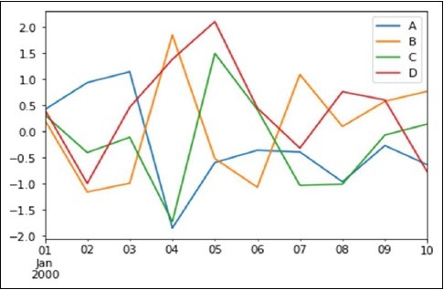
If the index consists of dates, then the pandas .plot() method calls the Matplotlib gct().autofmt_xdate() to format the x-axis labels.
Also we can plot one column versus another using the x and y keywords.
Types of Plots Available in Pandas
Pandas supports various plot types through the kind parameter or specialized plotting methods. Following is the overview of the different plotting methods −
| Plot Type | kind Value | Specialized Method | Use Case |
|---|---|---|---|
| Line | 'line' | .line() | Visualizing trends over time or a sequence. |
| Bar | 'bar' | .bar() | Comparing quantities across categories. |
| Horizontal Bar | 'barh' | .barh() | Same as bar charts, but horizontal. |
| Histogram | 'hist' | .hist() | Visualizing Distribution of numeric data. |
| Box Plot | 'box' | .box() | Summarizing data distribution and outliers. |
| Area | 'area' | .area() | Highlighting trends with cumulative data. |
| Scatter | 'scatter' | .scatter() | Relationship between two variables, for DataFrame only. |
| Hexbin | 'hexbin' | .hexbin() | Visualizing data density in two dimensions, for DataFrame only. |
| Density | 'kde' or 'density' | .kde() or .density() | Smoothing data distributions (Kernel Density Estimation). |
| Pie | 'pie' | .pie() | Proportional data in a circular graph. |
Example: Plotting Bar Plot with plot() method
Let us now see what a Bar Plot is by creating one. A bar plot can be created in the following way −
import pandas as pd import numpy as np import matplotlib.pyplot as plt # Creating a random DataFrame df = pd.DataFrame(np.random.rand(10,4), columns=['a','b','c','d']) # Plotting the bar plot df.plot(kind='bar') plt.show()
Output
Its output is as follows −
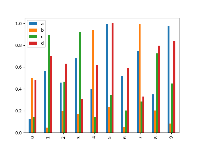
To produce a stacked bar plot, pass stacked=True −
import pandas as pd import numpy as np import matplotlib.pyplot as plt # Creating a random DataFrame df = pd.DataFrame(np.random.rand(10,4), columns=['a','b','c','d']) # Plotting the stacked Bar plot df.plot(kind='bar', stacked=True) plt.show()
Output
Its output is as follows −
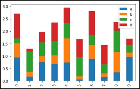
To get horizontal bar plots, use the barh option −
import pandas as pd import numpy as np import matplotlib.pyplot as plt # Creating a random DataFrame df = pd.DataFrame(np.random.rand(10,4), columns=['a','b','c','d']) # Plotting the horizontal bar plot df.plot(kind='barh', stacked=True) plt.show()
Output
Its output is as follows −

Histograms
Histograms can be plotted using the hist option of the plot() method kind argument. We can specify number of bins.
import pandas as pd
import numpy as np
import matplotlib.pyplot as plt
# Creating a random DataFrame
df = pd.DataFrame({'a':np.random.randn(1000)+1,'b':np.random.randn(1000),
'c':np.random.randn(1000) - 1}, columns=['a', 'b', 'c'])
df.plot(kind='hist', bins=20)
plt.show()
Output
Its output is as follows −
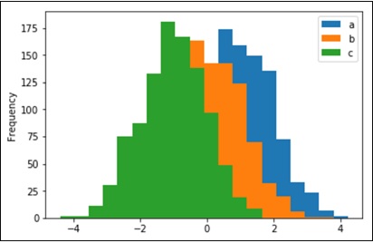
Box Plots
Box plot can be drawn calling 'box' option for both the Series and DataFrame objects to visualize the distribution of values within each column.
For instance, here is a boxplot representing five trials of 10 observations of a uniform random variable on [0,1).
import pandas as pd import numpy as np import matplotlib.pyplot as plt # Creating a random DataFrame df = pd.DataFrame(np.random.rand(10, 5), columns=['A', 'B', 'C', 'D', 'E']) df.plot(kind='box') plt.show()
Output
Its output is as follows −
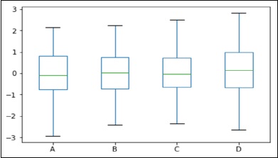
Area Plot
Area plot can be created using the plot(kind='area') option.
import pandas as pd import numpy as np import matplotlib.pyplot as plt # Creating a random DataFrame df = pd.DataFrame(np.random.rand(10, 4), columns=['a', 'b', 'c', 'd']) df.plot(kind='area') plt.show()
Output
Its output is as follows −
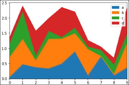
Scatter Plot
Scatter plot can be created using the plot(kind='scatter') option.
import pandas as pd import numpy as np import matplotlib.pyplot as plt # Creating a random DataFrame df = pd.DataFrame(np.random.rand(50, 4), columns=['a', 'b', 'c', 'd']) df.plot(kind='scatter', x='a', y='b') plt.show()
Output
Its output is as follows −
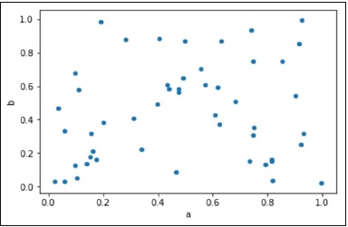
Pie Chart
Pie chart can be created using the plot(kind='pie') option.
import pandas as pd import numpy as np import matplotlib.pyplot as plt # Creating a random DataFrame df = pd.DataFrame(3 * np.random.rand(4), index=['a', 'b', 'c', 'd'], columns=['x']) df.plot(kind='pie', subplots=True) plt.show()
Output
Its output is as follows −
Python Pandas - Caveats & Gotchas
Caveats means warning and gotcha means an unseen problem.
Using If/Truth Statement with Pandas
Pandas follows the numpy convention of raising an error when you try to convert something to a bool. This happens in an if or when using the Boolean operations, and, or, or not. It is not clear what the result should be. Should it be True because it is not zerolength? False because there are False values? It is unclear, so instead, Pandas raises a ValueError −
import pandas as pd if pd.Series([False, True, False]): print 'I am True'
Output
Its output is as follows −
ValueError: The truth value of a Series is ambiguous. Use a.empty, a.bool() a.item(),a.any() or a.all().
In if condition, it is unclear what to do with it. The error is suggestive of whether to use a None or any of those.
import pandas as pd
if pd.Series([False, True, False]).any():
print("I am any")
Output
Its output is as follows −
I am any
To evaluate single-element pandas objects in a Boolean context, use the method .bool() −
import pandas as pd print pd.Series([True]).bool()
Output
Its output is as follows −
True
Bitwise Boolean
Bitwise Boolean operators like == and != will return a Boolean series, which is almost always what is required anyways.
import pandas as pd s = pd.Series(range(5)) print s==4
Output
Its output is as follows −
0 False 1 False 2 False 3 False 4 True dtype: bool
isin Operation
This returns a Boolean series showing whether each element in the Series is exactly contained in the passed sequence of values.
import pandas as pd
s = pd.Series(list('abc'))
s = s.isin(['a', 'c', 'e'])
print s
Output
Its output is as follows −
0 True 1 False 2 True dtype: bool
Reindexing vs ix Gotcha
Many users will find themselves using the ix indexing capabilities as a concise means of selecting data from a Pandas object −
import pandas as pd
import numpy as np
df = pd.DataFrame(np.random.randn(6, 4), columns=['one', 'two', 'three',
'four'],index=list('abcdef'))
print df
print df.ix[['b', 'c', 'e']]
Output
Its output is as follows −
one two three four
a -1.582025 1.335773 0.961417 -1.272084
b 1.461512 0.111372 -0.072225 0.553058
c -1.240671 0.762185 1.511936 -0.630920
d -2.380648 -0.029981 0.196489 0.531714
e 1.846746 0.148149 0.275398 -0.244559
f -1.842662 -0.933195 2.303949 0.677641
one two three four
b 1.461512 0.111372 -0.072225 0.553058
c -1.240671 0.762185 1.511936 -0.630920
e 1.846746 0.148149 0.275398 -0.244559
This is, of course, completely equivalent in this case to using the reindex method −
import pandas as pd
import numpy as np
df = pd.DataFrame(np.random.randn(6, 4), columns=['one', 'two', 'three',
'four'],index=list('abcdef'))
print df
print df.reindex(['b', 'c', 'e'])
Output
Its output is as follows −
one two three four
a 1.639081 1.369838 0.261287 -1.662003
b -0.173359 0.242447 -0.494384 0.346882
c -0.106411 0.623568 0.282401 -0.916361
d -1.078791 -0.612607 -0.897289 -1.146893
e 0.465215 1.552873 -1.841959 0.329404
f 0.966022 -0.190077 1.324247 0.678064
one two three four
b -0.173359 0.242447 -0.494384 0.346882
c -0.106411 0.623568 0.282401 -0.916361
e 0.465215 1.552873 -1.841959 0.329404
Some might conclude that ix and reindex are 100% equivalent based on this. This is true except in the case of integer indexing. For example, the above operation can alternatively be expressed as −
import pandas as pd
import numpy as np
df = pd.DataFrame(np.random.randn(6, 4), columns=['one', 'two', 'three',
'four'],index=list('abcdef'))
print df
print df.ix[[1, 2, 4]]
print df.reindex([1, 2, 4])
Output
Its output is as follows −
one two three four
a -1.015695 -0.553847 1.106235 -0.784460
b -0.527398 -0.518198 -0.710546 -0.512036
c -0.842803 -1.050374 0.787146 0.205147
d -1.238016 -0.749554 -0.547470 -0.029045
e -0.056788 1.063999 -0.767220 0.212476
f 1.139714 0.036159 0.201912 0.710119
one two three four
b -0.527398 -0.518198 -0.710546 -0.512036
c -0.842803 -1.050374 0.787146 0.205147
e -0.056788 1.063999 -0.767220 0.212476
one two three four
1 NaN NaN NaN NaN
2 NaN NaN NaN NaN
4 NaN NaN NaN NaN
It is important to remember that reindex is strict label indexing only. This can lead to some potentially surprising results in pathological cases where an index contains, say, both integers and strings.